CS-250 Algorithms
- Links and books
- Analyzing algorithms
- Sorting
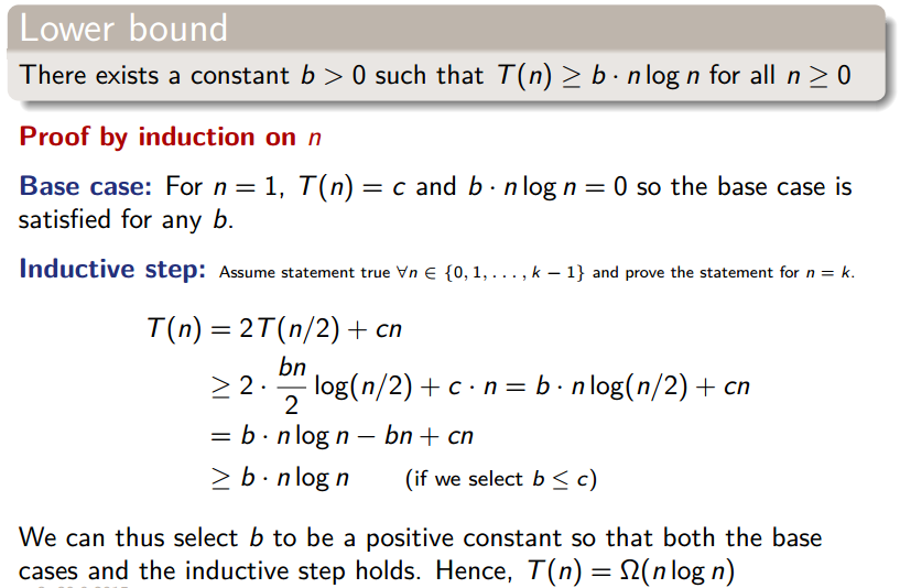
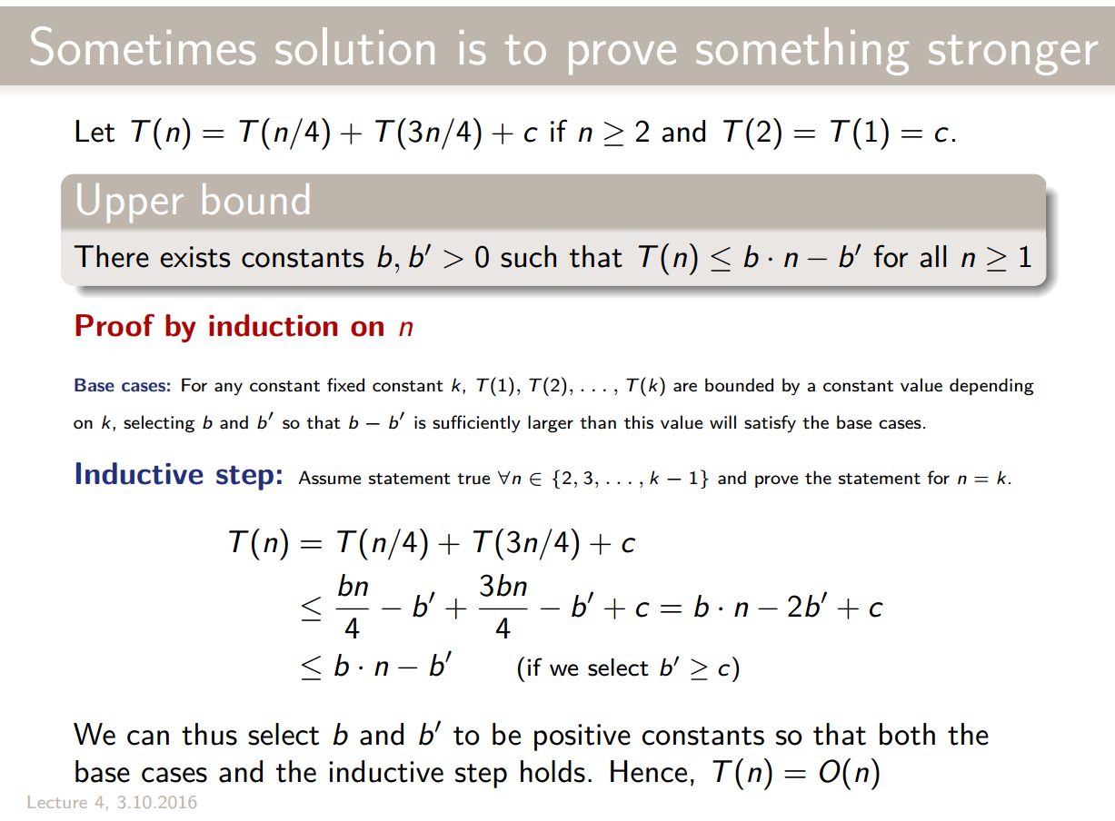
- Recurrences
- Maximum-Subarray Problem
- Matrix multiplication
- Heaps and Heapsort
- More data structures
- Dynamic Programming
- Graphs
- Flow Networks
- Data structures for disjoint sets
- Minimum Spanning Trees (MST)
- Shortest Path Problem
- Probabilistic analysis and randomized algorithms
- Quick Sort
- Review of the course
Links and books
- Course homepage
- Introduction to Algorithms, Third edition (2009), T. Cormen, C. Lerserson, R. Rivest, C. Stein (book on which the course is based)
- The Art of Computer Programming, Donald Knuth (a classic)
Analyzing algorithms
We’ll work under a model that assumes that:
- Instructions are executed one after another
- Basic instructions (arithmetic, data movement, control) take constant O(1) time
- We don’t worry about numerical precision, although it is crucial in certain numerical applications
We usually concentrate on finding the worst-case running time. This gives a guaranteed upper bound on the running time. Besides, the worst case often occurs in some algorithms, and the average is often as bad as the worst-case.
Sorting
The sorting problem’s definition is the following:
- Input: A sequence of numbers
- Output: A permutation (reordering) of the input sequence in increasing order
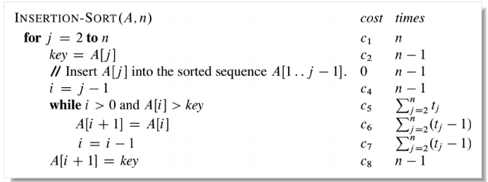
Insertion sort
This algorithm works somewhat in the same way as sorting a deck of cards. We take a single element and traverse the list to insert it in the right position. This traversal works by swapping elements at each step.
1
2
3
4
5
6
7
8
9
10
11
12

def insertion_sort(A, n):
    # We start at 2 because a single element is already sorted.
    # The upper bound in range is exclusive, so we set it to n+1
    for j in range(2, n+1):
        key = A[j]
        # Insert A[j] in to the sorted sequence A[1..j-1]
        i = j-1
        while i > 0 and A[i] > key:
            # swap
            A[i+1] = A[i]
            i = i-1
        A[i+1] = key
Correctness
Using induction-like logic.
Loop invariant: At the start of each iteration of the “outer” for loop — the loop indexed by j — the subarray A[1, ..., j-1] consists of the elements originally in A[1, ..., j-1] but in sorted order.
We need to verify:
-
Initialization: We start at
j=2so we start with one element. One number is trivially sorted compared to itself. -
Maintenance: We’ll assume that the invariant holds at the beginning of the iteration when
j=k. The body of theforloop works by movingA[k-1],A[k-2]ansd so on one step to the right until it finds the proper position forA[k]at which points it inserts the value ofA[k]. The subarrayA[1..k]then consists of the elements in a sorted order. Incrementingjtok+1preserves the loop invariant. -
Termination: The condition of the
forloop to terminate is thatj>n; hence,j=n+1when the loop terminates, andA[1..n]contains the original elements in sorted order.
Analysis
- Best case: The array is already sorted, and we can do
- Worst case: The array is sorted in reverse, so and the algorithm runs in :
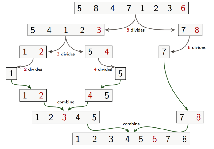
Merge Sort
Merge sort is a divide-and-conquer algorithm:
- Divide the problem into a number of subproblems that are smaller instances of the same problem
- Conquer the subproblems by solving them recursively. Base case: If the subproblems are small enough, just solve them by brute force
- Combine the subproblem solutions to give a solution to the original problem
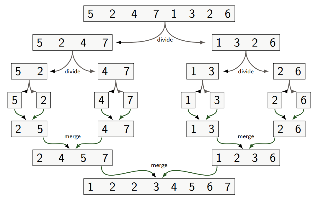
Merge sort can be implemented recursively as such:
1
2
3
4
5
6
7
8
9
10
11
12
13
14
15
16
17
18
19
20
21
22
23
24
25
26
27

def merge_sort(A, p, r):
    if p < r: # Check for base case
        q = math.floor((p + r) / 2) # Divide
                                    # q is the index at which we split the list
        merge_sort(A, p, q) # Conquer
        merge_sort(a, q+1, r) # Conquer
        merge(A, p, q, r) # Combine

def merge(A, p, q, r):
    n1 = q - p + 1 # Size of the first half
    n2 = r - q # Size of the second half
    let L[1 .. n1 + 1] and R[1 .. n2 + 1] be new arrays
    for i = 1 to n1:
        L[i] = A[p + i - 1]
    for j = 1 to n2:
        R[j] = A[q + j]
    L[n1 + 1] = infinity # in practice you could use sys.maxint
    R[n2 + 1] = infinity
    i = 1
    j = 1
    for k = p to r:
        if L[i] <= R[j]:
            A[k] = L[i]
            i = i + 1
        else:
            A[k] = R[j]
            j = j + 1
In the merge function, instead of checking whether either of the two lists that we’re merging is empty, we can just add a sentinel to the bottom of the list, with value ∞. This works because we’re just picking the minimum value of the two.
This algorithm works well in parallel, because we can split the lists on separate computers.
Correctness
Assuming merge is correct, we can do a proof by strong induction on .
-
Base case, : In this case so
A[p..r]is trivially sorted. -
Inductive case: By induction hypothesis
merge_sort(A, p, q)andmerge_sort(A, q+1, r)successfully sort the two subarrays. Therefore a correct merge procedure will successfully sortA[p..q]as required.
Recurrences
Let’s try to provide an analysis of the runtime of merge sort.
- Divide: Takes contant time, i.e.,
- Conquer: Recursively solve two subproblems, each of size , so we create a problem of size for each step.
- Combine: Merge on an n-element subarray takes time, so
Our recurrence therefore looks like this:
Trying to substitue multiple times yields . By now, a qualified guess would be that . We’ll prove this the following way:
All-in-all, merge sort runs in , both in worst and best case.
For small instances, insertion sort can still be faster despite its quadratic runtime; but for bigger instances, merge sort is definitely faster.
However, merge sort is not in-place, meaning that it does not operate directly on the list that needs to be sorted, unlike insertion sort.
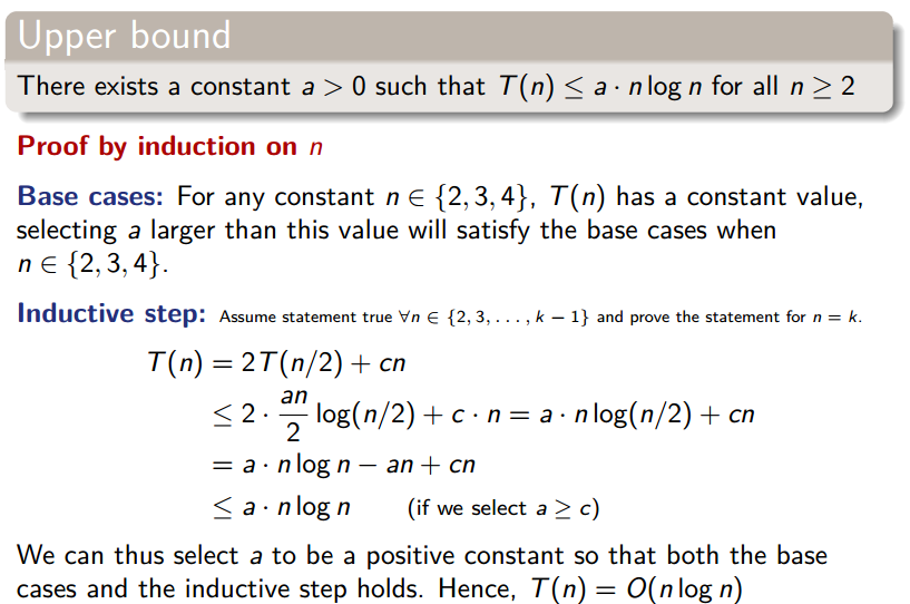
Master Theorem
Generally, we can solve recurrences in a black-box manner thanks to the Master Theorem:
Let and be constants, let be defined on the nonnegative integers by the recurrence:
Then, has the following asymptotic bounds
- If for some constant , then
- If , then
- If for some constant , and if for some constant and all sufficiently large , then
The 3 cases correspond to the following cases in a recursion tree:
- Leaves dominate
- Each level has the same cost
- Roots dominate
Maximum-Subarray Problem
Description
You have the prices that a stock traded at over a period of n consecutive days. When should you have bought the stock? When should you have sold the stock?
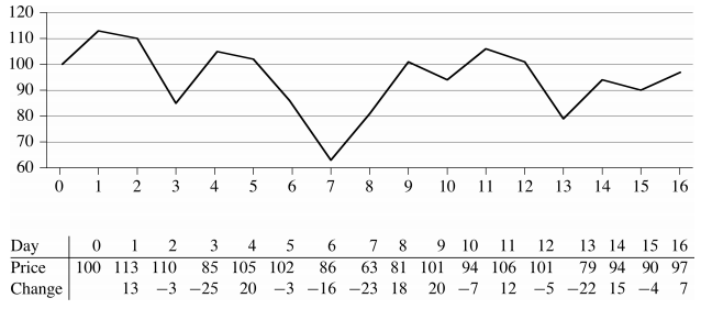
The naïve approach of buying at the all-time lowest and selling at the all-time highest won’t work, as the lowest price might occur after the highest.
We describe the problem as follows:
-
Input: An array
A[1..n]of price changes -
Output: Indices
iandjsuch thatA[i..j]has the greatest sum of any nonempty, contiguous subarray ofA, along with the sum of the values inA[i..j]
Note that the array A could be price changes prices on each day, the two problems are equivalent (and can be converted into each other in linear time). In the first case, profit is sum(A[i..j]), while in the second the profit is A[j] - A[i]. We will be talking about this problem in the first form, with the price changes.
We can also decide to allow or disallow buying and selling on the same day, which would give us 0 profit. In other words, this would be disallowing empty maximum subarrays. We’ll first see a variant which disallows it, and then a variant which allows it.
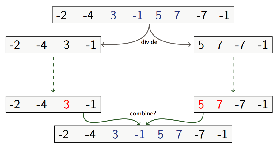
Divide and Conquer
-
Divide the subarray into two subarrays of as equal size as possible: Find the midpoint mid of the subarrays, and consider the subarrays
A[low..mid]andA[mid+1..high]- This can run in
-
Conquer by finding maximum subarrays of
A[low..mid]andA[mid+1..high]- Recursively solve two subproblems, each of size , so
-
Combine: Find a maximum subarray that crosses the midpoint, and use the best solution out of the three (that is, left, midpoint and right).
- The merge is dominated by
find_max_crossing_subarrayso
- The merge is dominated by
The overall recursion is , so the algorithm runs in .
In pseudo-code the algorithm is:
1
2
3
4
5
6
7
8
9
10
11
12
13
14
15
16
17
18
19
20
21
22
23
24
25
26
27
28
29
30
31
32
33
34
35
36
37
38

def find_maximum_subarray(A, low, high):
    if high == low: # base case: only one element
        return (low, high, A[low])
    else:
        mid = math.floor((low + high)/2)
        (l_low, l_high, l_sum) = find_maximum_subarray(A, low, mid)
        (r_low, r_high, r_sum) = find_maximum_subarray(A, mid+1, high)
        (x_low, x_high, x_sum) = find_max_crossing_subarray(A, low, mid, high)

        # Find the best solution of the three:
        if l_sum >= r_sum and l_sum >= x_sum:
            return (l_low, l_high, l_sum)
        elif r_sum >= l_sum and r_sum >= x_sum:
            return (r_low, r_high, r_sum)
        else:
            return (x_low, x_high, x_sum)

def find_max_crossing_subarray(A, low, mid, high):
    # Find a maximum subarray of the form A[i..mid]
    l_sum = - infinity # Lower-bound sentinel
    sum = 0
    for (i = mid) downto low:
        sum += A[i]
        if sum > l_sum:
            l_sum = sum
            l_max = i

    # Find a maximum subarray of the form A[mid+1..j]
    r_sum = - infinity # Lower-bound sentinel
    sum = 0
    for j = mid to high:
        sum += A[j]
        if sum > r_sum:
            r_sum = sum
            r_max = j

    # Return the indices and the sum of the two subarrays
    return (l_max, r_max, l_sum + r_sum)
Improvement with Dynamic Programming
The divide-and-conquer algorithm can be improved to , which is optimal. This algorithm is known as Kadane’s algorithm. For the sake of simplicity, we won’t keep track of indices in this variant, but we could extend it to do so (see Wikipedia article). Also note that we will be looking at the variant of the problem which allows empty maximum subarrays (but it can be easily adapted to disallow it, see Wikipedia article).
1
2
3
4
5
6
7

def find_max_subarray(A: List[int]) -> int:
    best_sum = 0
    current_sum = 0
    for x in A:
        current_sum = max(0, current_sum + x)
        best_sum = max(best_sum, current_sum)
    return best_sum
This is a “simple” example of dynamic programming, which we’ll talk more about later. It is “simple” because we don’t actually need memoization, as each subproblem only needs to be computed once. But it can still be useful to think of it in DP terms. We can describe the DP recursion as follows, where the array contains the sum of the maximum subarray ending at (or in terms of our stock market analogy, the profit made if we sell on day ):
Let’s try to get an intuitive sense for what the recursion says. To compute the maximum subarray ending at , we can either extend the max subarray ending at to include day , or if that makes us lose money, we can say that the best way to sell on day is to also buy on day (which gives us 0 profit).
Why is this valid? The above recursion has an important property: holds the maximum over all of the sum . In other words, it holds the max sum for a subarray starting anywhere before (or at ) and ending at .
By returning the max value contained in , we then have the maximum subarray.
The recursion also nicely shows that each index in the recursion only uses the index before, which gives us an easy way to construct a bottom-up variant of the algorithm. We can translate the recursion to the loop invariant that is true for Kadane’s algorithm: at the beginning of step , current_sum holds the value of the maximum subarray ending at .
This is all an exercise in how to think of this problem, because if we are given the list of prices rather than the list of changes, it may be more intuitive to see how we can solve this:
1
2
3
4
5
6
7

def find_max_profit(prices: List[int]) -> int:
    min_price = float("inf")
    max_profit = 0
    for price in prices:
        min_price = min(price, min_price)
        max_profit = max(max_profit, price - min_price)
    return max_profit
Matrix multiplication
- Input: Two (square) matrices, and
- Output: matrix where .
Naive Algorithm
The naive algorithm simply calculates . It runs in and uses space.
We can do better.
Divide-and-Conquer algorithm
- Divide each of A, B and C into four matrices so that:
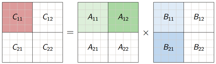
-
Conquer: We can recursively solve 8 matrix multiplications that each multiply two matrices, since:
- .
- .
-
Combine: Make the additions to get to C.
- is .
Pseudocode and analysis
1
2
3
4
5
6
7
8
9
10

def rec_mat_mult(A, B, n):
    let C be a new n*n matrix
    if n == 1:
        c11 = a11 * b11
    else partition A, B, and C into n/2 * n/2 submatrices:
        C11 = rec_mat_mult(A[1][1], B[1][1], n/2) + rec_mat_mult(A[1][2], B[2][1], n/2)
        C12 = rec_mat_mult(A[1][1], B[1][2], n/2) + rec_mat_mult(A[1][2], B[2][2], n/2)
        C21 = rec_mat_mult(A[2][1], B[1][1], n/2) + rec_mat_mult(A[2][2], B[2][1], n/2)
        C22 = rec_mat_mult(A[2][1], B[1][2], n/2) + rec_mat_mult(A[2][2], B[2][2], n/2)
    return C
The whole recursion formula is . So we did all of this for something that doesn’t even beat the naive implementation!!
Strassen’s Algorithm for Matrix Multiplication
What really broke the Divide-and-Conquer approach is the fact that we had to do 8 matrix multiplications. Could we do fewer matrix multiplications by increasing the number of additions?
Spoiler Alert: Yes.
There is a way to do only 7 recursive multiplications of matrices, rather than 8. Our recurrence relation is now:
Strassen’s method is the following:
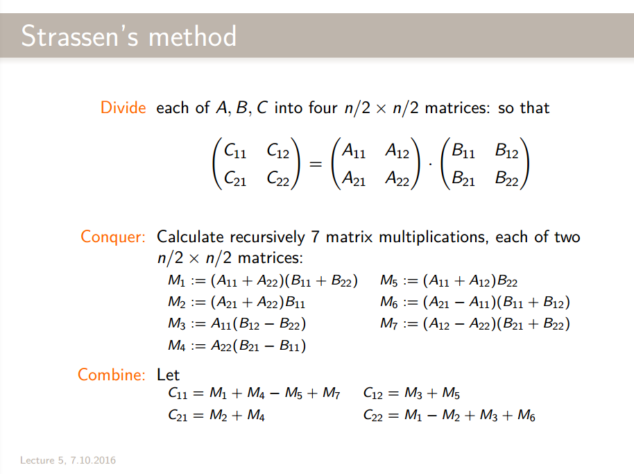
Note that when our matrix’s size isn’t a power of two, we can just pad our operands with zeros until we do have a power of two size. This still runs in .
Notes about Strassen
- First to beat time
- Faster methods are known today: Coppersmith and Winograd’s method runs in time , which has recently been improved by Vassilevska Williams to .
- How to multiply matrices in best way is still a big open problem
- The naive method is better for small instances because of hidden constants in Strassen’s method’s runtime.
Heaps and Heapsort
Heaps
A heap is a nearly complete binary tree (meaning that the last level may not be complete). In a max-heap, the maximum element is at the root, while the minimum element takes that place in a min-heap.
We can store the heap in a list, where each element stores the value of a node:
-
RootisA[1] -
Left(i)is2i -
Right(i)is2i + 1 -
Parent(i)isfloor(i/2)
The main property of a heap is:
A heap rooted at position i in an array satisfies the heap property if:
-
Max-heap: the key of
i’s children is smaller or equal toi’s key. -
Min-heap: the key of
i’s children is greater or equal toi’s key.
In a heap, all nodes satisfy the heap property. Note that this does not mean that a heap is fully ordered. It has some notion of order, in that children are smaller or equal to their parent, but no guarantee is made about values in the left subtree compared to those in the right subtree.
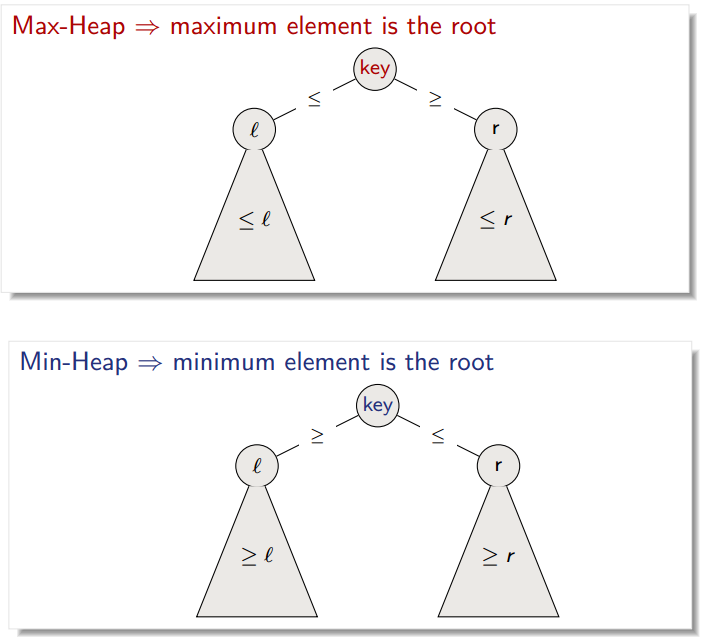
A good way to understand a heap is to say that if you pick a path through the heap from root to leaf and traverse it, you are guaranteed to see numbers in decreasing order for a max-heap, and increasing order for a min-heap.
The height of a node is the number of edges on a longest simple path from the node down to a leaf. The height of the heap is therefore simply the height of the root, .
Max-Heapify
It’s a very important algorithm for manipulating heaps. Given an i such that the subtrees of i are heaps, it ensures that the subtree rooted at i is a heap satisfying the heap property. The outline is as follows:
- Compare
A[i],A[Left(i)],A[Right(i)] - If necessary, swap
A[i]with the largest of the two children to preserve heap property. - Continue this process of comparing and swapping down the heap, until the subtree rooted at i is a max-heap.
1
2
3
4
5
6
7
8
9
10
11
12
13
14
15
16
17
18
19
20
21
22
23
24
25
26
27

def max_heapify(A: List[int], i: int, n: int):
    """
    Modifies `A` in-place so that the node at `i` roots a heap.

    A : List in which the left and right children of `i` root heaps
        (but `i` may not)
    i : Index of the node which we want to heapify
    n : Length of `A`
    """
    l = Left(i)
    r = Right(i)

    # Pick larger of left (if it exists) and parent:
    if l <= n and A[l] > A[i]:
        largest = l
    else:
        largest = i

    # Pick larger of right (if it exists) and current largest:
    if r <= n and A[r] > A[largest]:
        largest = r

    # If the root isn't already the largest, swap the root with the
    # largest:
    if largest != i:
        swap A[i] and A[largest]
        max_heapify(A, largest, n)
This runs in and uses space.
What may be surprising is that we only recurse when the node at i isn’t the largest; but remember that A is already such that the left and right subtrees of i already satisfy the heap property; they are already the roots of heaps. If i is larger than both left and right, then we preserve the heap property. If not, we may have to recursively modify one subtree to preserve the property.
Building a heap
Given an unordered array A of length n, build_max_heap outputs a heap.
1
2
3
4
5
6
7
8
9

def build_max_heap(A: List[int], n: int):
    """
    Modifies `A` in-place so that `A` becomes a heap.

    A : List of numbers
    n : Length of `A`
    """
    for i = floor(n/2) downto 1:
        max_heapify(A, i, n)
This procedure operates in-place. We can start at since all elements after that threshold are leaves, so we’re not going to heapify those anyway. Note that the node index i decreases, meaning that we’re generally going upwards in the tree. This is on purpose, as max_heapify may go back downwards in order to push small elements down to the bottom of the heap.
We have calls to max_heapify, each of which takes time, so we have in total.
However, we can give a tighter bound: the time to run max_heapify is linear in the height of the node it’s run on. Hence, the time is bounded by:
Which is , since:
See the slides for a proof by induction.
Heapsort
Heapsort is the best of both worlds: it’s like merge sort, and sorts in place like insertion sort.
- Starting with the root (the maximum element), the algorithm places the maximum element into the correct place in the array by swapping it with the element in the last position in the array.
- “Discard” this last node (knowing that it is in its correct place) by
decreasing the heap size, and calling
max_heapifyon the new (possibly incorrectly-placed) root. - Repeat this “discarding” process until only one node (the smallest element) remains, and therefore is in the correct place in the array
1
2
3
4
5

def heapsort(A, n):
    build_max_heap(A, n)
    for i = n downto 2:
        exchange A[1] with A[i]
        max_heapify(A, 1, i-1)
-
build_max_heap: -
forloop: times - Exchange elements:
-
max_heapify:
Total time is therefore .
Priority queues
In a priority queue, we want to be able to:
- Insert elements
- Find the maximum
- Remove and return the largest element
- Increase a key
A heap efficiently implements priority queues.
Finding maximum element
This can be done in by simply returning the root element.
1
2

def heap_maximum(A):
    return A[1]
Extracting maximum element
We can use max heapify to rebuild our heap after removing the root. This runs in , as every other operation than max-heapify runs in .
1
2
3
4
5
6
7
8

def heap_extract_max(A, n):
    if n < 1: # Check that the heap is non-empty
        error "Heap underflow"
    max = A[1]
    A[1] = A[n] # Make the last node in the tree the new root
    n = n - 1 # Remove the last node of the tree
    max_heapify(A, 1, n) # Re-heapify the heap
    return max
Increasing a value
1
2
3
4
5
6
7
8
9

def heap_increase_key(A, i, key):
    if key < A[i]:
        error "new key is smaller than current key"
    A[i] = key
    # Traverse the tree upward comparing new key to parent and swapping keys
    # if necessary, until the new key is smaller than the parent's key:
    while i > 1 and A[Parent(i)] < A[i]:
        exchange A[i] with A[Parent(i)]
        i = Parent(i)
This traverses the tree upward, and runs in .
Inserting into the heap
1
2
3
4

def max_heap_insert(A, key, n):
    n = n + 1 # Increment the size of the heap
    A[n] = - infinity # Insert a sentinel node in the last pos
    heap_increase_key(A, n, key) # Increase the value to key
We know that this runs in the time for heap_increase_key, which is .
Summary
- Heapsort runs in and is in-place. However, a well implemented quicksort usually beats it in practice.
- Heaps efficiently implement priority queues:
-
insert(S, x): -
maximum(S): -
extract_max(S): -
increase_key(S, x, k):
-
More data structures
Stacks
Stacks are LIFO (last-in, first out). It has two basic operations:
- Insertion with
push(S, x) - Delete operation with
pop(S)
We can implement a stack using an array where S[1] is the bottom element, and S[S.top] is the element at the top.
1
2
3
4
5
6
7
8
9
10
11
12
13
14
15

def stack_empty(S):
    if S.top = 0:
        return true
    else return false

def push(S, x):
    S.top = S.top + 1 # Increment the pointer to the top
    S[S.top] = x # Store element

def pop(S):
    if stack_empty(S):
        error "underflow"
    else
        S.top = S.top - 1 # Decrement the pointer to the top
        return S[S.top + 1] # Return what we've removed
These operations are all .
Queues
Queues are FIFO (first-in, first-out). They have two basic operations:
- Insertion with
enqueue(Q, x) - Deletion with
dequeue(Q)
Again, queues can be implemented using arrays with two pointers: Q[Q.head] is the first element, Q[Q.tail] is the next location where a newly arrived element will be placed.
1
2
3
4
5
6
7
8
9
10
11
12
13

def enqueue(Q, x):
    Q[Q.tail = x]
    # Now, update the tail pointer:
    if Q.tail = Q.length: # Q.length is the length of the array
        Q.tail = 1 # Wrap it around
    else Q.tail = Q.tail + 1

def dequeue(Q):
    x = Q[Q.head]
    # Now, update the head pointer
    if Q.head = Q.length:
        Q.head = 1
    else Q.head = Q.head + 1
Notice that we’re not deleting anything per se. We’re just moving the boundaries of the queue and sometimes replacing elements.
Positives:
- Very efficient
- Natural operations
Negatives:
- Limited support: for example, no search
- Implementations using arrays have fixed capacity
Linked Lists
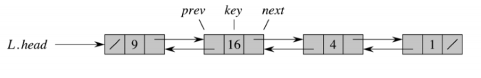
/ symbol represents Nil.Let’s take a look at the operations in linked lists.
Search
1
2
3
4
5

def list_search(L, k):
    x = L.head
    while x != nil and x.key != k:
        x = x.next
    return x
This runs in . If no element with key k exists, it will return nil.
Insertion
1
2
3
4
5
6

def list_insert(L, x):
    x.next = L.head
    if L.head != nil:
        L.head.prev = x
    L.head = x # Rewrite the head pointer
    x.prev = nil
This runs in . This linked list doesn’t implement a tail pointer, so it’s important to add the element to the start of the list and not the end, as that would mean traversing the list before adding the element.
Deletion
1
2
3
4
5
6

def list_delete(L, x):
    if x.prev != nil:
        x.prev.next = x.next
    else L.head = x.next
    if x.next != nil:
        x.next.prev = x.prev
This is .
Summary
- Insertion:
- Deletion:
- Search:
Search in linear time is no fun! Let’s see how else we can do this.
Binary search trees
The key property of binary search trees is:
- If
yis in the left subtree ofx, theny.key < x.key - If
yis in the right subtree ofx, theny.key >= x.key
The tree T has a root T.root, and a height h (not necessarily log(n), it can vary depending on the organization of the tree).
Querying a binary search tree
All of the following algorithms can be implemented in .
Searching
1
2
3
4
5
6
7

def tree_search(x, k):
    if x == None or k == x.key:
        return x
    if k < x.key:
        return tree_search(x.left, k)
    else:
        return tree_search(x.right, k)
Maximum and minimum
By the key property, the minimum is in the leftmost node, and the maximum in rightmost.
1
2
3
4
5
6
7
8
9

def tree_minimum(x):
    while x.left != None:
        x = x.left
    return x

def tree_maximum(x):
    while x.right != None:
        x = x.right
    return x
Successor
The successor or a node x is the node y such that y.key is the smallest key that is strictly larger than x.key.
There are 2 cases when finding the successor of x:
-
xhas a non-empty right subtree:x’s successor is the minimum in the right subtree -
xhas an empty right subtree: We go left up the tree as long as we can (until nodey), and andx’s successor is the parent ofy(oryif it is the root)
1
2
3
4
5
6
7
8

def tree_successor(x):
    if x.right != None:
        return tree_minimum(x.right)
    y = x.parent
    while y != None and x == y.right:
        x = y
        y = y.parent
    return y
In the worst-case, this will have to traverse the tree upward, so it indeed runs in .
Printing a binary search tree
Let’s consider the following tree:
Inorder
- Print left subtree recursively
- Print root
- Print right subtree recursively
1
2
3
4
5

def inorder_tree_walk(x):
    if x != None:
        inorder_tree_walk(x.left)
        print x.key
        inorder_tree_walk(x.right)
This would print:
1, 2, 3, 4, 5, 6, 7, 8, 9 10, 11, 12This runs in .
Proof of runtime
We have runtime of inorder_tree_walk on a tree with nodes.
Base:
Induction: Suppose that the tree rooted at has nodes in its left subtree, and nodes in the right.
Therefore:
Therefore, we do indeed have .
Preorder and postorder follow a very similar idea.
Preorder
- Print root
- Print left subtree recursively
- Print right subtree recursively
1
2
3
4
5

def inorder_tree_walk(x):
    if x != None:
        print x.key
        inorder_tree_walk(x.left)
        inorder_tree_walk(x.right)
This would print:
8, 4, 2, 1, 3, 6, 5, 12, 10, 9, 11Postorder
- Print left subtree recursively
- Print right subtree recursively
- Print root
1
2
3
4
5

def inorder_tree_walk(x):
    if x != None:
        inorder_tree_walk(x.left)
        inorder_tree_walk(x.right)
        print x.key
This would print:
1, 3, 2, 5, 6, 4, 9, 11, 10, 12, 8Modifying a binary seach tree
The data structure must be modified to reflect the change, but in such a way that the binary-search-tree property continues to hold.
Insertion
- Search for
z.key - When arrived at
Nilinsertzat that position
1
2
3
4
5
6
7
8
9
10
11
12
13
14
15
16
17
18
19

def tree_insert(T, z):
    # Search phase:
    y = None
    x = T.root
    while x != None:
        y = x
        if z.key < x.key:
            x = x.left
        else:
            x = x.right
    z.parent = y

    # Insert phase
    if y == Nil:
        T.root = z # Tree T was empty
    elsif z.key < y.key:
        y.left = z
    else:
        y.right = z
This runs in .
Deletion
Conceptually, there are 3 cases:
- If
zhas no children, remove it - If
zhas one child, then make that child takez’s position in the tree - If
zhas two children, then find its successoryand replacezbyy
1
2
3
4
5
6
7
8
9
10
11
12
13
14
15
16
17
18
19
20
21
22
23
24
25
26
27
28
29

# Replaces subtree rooted at u with that rooted at v
def transplant(T, u, v):
    if u.parent == Nil: # If u is the root
        T.root = v
    elsif u == u.parent.left: # If u is to the left
        u.parent.left = v
    else: # If u is to the right
        u.parent.right = v
    if v != Nil: # If v isn't the root
        v.parent = u.parent

# Deletes the subtree rooted at z
def tree_delete(T, z):
    if z.left == Nil: # z has no left child
        transplant(T, z, z.right) # move up the right child
    if z.right == Nil: # z has just a left child
        transplant(T, z, z.left) # move up the left child
    else: # z has two children
        y = tree_minimum(z.right) # y is z's successor
        if y.parent != z:
            # y lies within z's right subtree but not at the root of it
            # We must therefore extract y from its position
            transplant(T, y, y.right)
            y.right = z.right
            y.right.parent = y
        # Replace z by y:
        transplant(T, z, y)
        y.left = z.left
        y.left.parent = y
Summary
- Query operations: Search, max, min, predecessor, successor:
- Modifying operations: Insertion, deletion:
There are efficient procedures to keep the tree balanced (AVL trees, red-black trees, etc.).
Summary
- Stacks: LIFO, insertion and deletion in , with an array implementation with fixed capacity
- Queues: FIFO, insertion and deletion in , with an array implementation with fixed capacity
- Linked Lists: No fixed capcity, insertion and deletion in , supports search but time.
- Binary Search Trees: No fixed capacity, supports most operations (insertion, deletion, search, max, min) in time .
Dynamic Programming
The main idea is to remember calculations already made. This saves enormous amounts of computation, as we don’t have to do the same calculations again and again.
There are two different ways to implement this:
Top-down with memoization
Solve recursively but store each result in a table. Memoizing is remembering what we have computed previously.
As an example, let’s calculate Fibonacci numbers with this technique:
1
2
3
4
5
6
7
8
9
10
11
12
13
14

def memoized_fib(n):
    let r = [0...n] be a new array
    for i = 0 to n:
        r[i] = - infinity # Initialize memory to -inf
    return memoized_fib_aux(n, r)

def memoized_fib_aux(n, r):
    if r[n] >= 0:
        return r[n]
    if n == 0 or n == 1:
        ans = 1
    else ans = memoized_fib_aux(n-1, r) + memoized_fib_aux(n-2, r)
    r[n] = ans
    return r[n]
This runs in .
Bottom-up
Sort the subproblems and solve the smaller ones first. That way, when solving a subproblem, we have already solved the smaller subproblems we need.
As an example, let’s calculate Fibonacci numbers with this technique:
1
2
3
4
5
6
7

def bottom_up_fib(n):
    let r = [0 ... n] be a new array
    r[0] = 1
    r[1] = 1
    for i = 2 to n:
        r[i] = r[i-1] + r[i-2]
    return r[n]
This is also .
Rod cutting problem
The instance of the problem is:
- A length of a metal rods
- A table of prices for rods of lengths
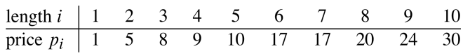
The objective is to decide how to cut the rod into pieces and maximize the price.
There are possible solutions (not considering symmetry), so we can’t just try them all. Let’s introduce the following theorem in an attempt at finding a better way:
Structural Theorem
If:
- The leftmost cut in an optimal solution is after units
- An optimal way to cut a solution of size is into rods of sizes
Then, an optimal way to cut our rod is into rods of size .
Essentially, the theorem say that to obtain an optimal solution, we need to cut the remaining pieces in an optimal way. This is the optimal substructure property. Hence, if we let be the optimal revenue from a rod of length , we can express recursively as follows:
Algorithm
Let’s try to implement a first algorithm. This is a direct implementation of the recurrence relation above:
1
2
3
4
5
6
7

def cut_rod(p, n):
    id n == 0:
        return 0
    q = -inf
    for i = 1 to n:
        q = max(q, p[i] + cut_rod(p, n-i))
    return q
But implementing this, we see that it isn’t terribly efficient — in fact, it’s exponential. Let’s try to do this with dynamic programming. Here, we’ll do it in a memoized top-down approach.
1
2
3
4
5
6
7
8
9
10
11
12
13
14
15
16

def memoized_cut_rod(p, n):
    let r[0..n] be a new array
    Initialize all entries to -infinity
    return memoized_cut_rod_aux(p, n, r)

def memoized_cut_rod_aux(p, n, r):
    if r[n] >= 0: # if it has been calculated
        return r[n]
    if n == 0:
        q = 0
    else:
        q = - infinity
        for i = 1 to r:
            q = max(q, p[i] + memoized_cut_rod_aux(p, n-i, r))
    r[n] = q
    return q
Every problem needs to check all the subproblems. Thanks to dynamic programming, we can just sum them instead of multiplying them, as every subproblem is computed once at most. As we’ve seen earlier on with insertion sort, this is:
The total time complexity is . This is even clearer with the bottom up approach:
1
2
3
4
5
6
7
8
9

def bottom_up_cut_rod(p, n):
    let r[0..n] be a new array
    r[0] = 0
    for j = 1 to n:
        q = - infinity
        for i = 1 to j:
            q = max(q, p[i]+ r[j -1])
        r[j] = q
    return r[n]
There’s a for-loop in a for-loop, so we clearly have .
Top-down only solves the subproblems actually needed, but recursive calls introduce overhead.
Extended algorithm
1
2
3
4
5
6
7
8
9
10
11
12
13
14
15
16
17
18
19

def extended_bottom_up_cut_rod(p, n):
    let r[0..n] and s[0..n] be new arrays
    # r[n] will be the price you can get for a rod of length n
    # s[n] the cuts of optimum location for a rod of length n
    r[0] = 0
    for j = 1 to n:
        q = -infinity
        for i to j:
            if q < p[i] + r[j-i]: # best cut so far?
                q = p[i] + r[j-i] # save its price
                s[j] = i # and save the index!
    r[j] = q
    return (r, s)

def print_cut_rod_solution(p, n):
    (r, s) = extended_bottom_up_cut_rod(p, n)
    while n > 0:
        print s[n]
        n = n - s[n]
When can dynamic programming be used?
- Optimal substructure
- An optimal solution can be built by combining optimal solutions for the subproblems
- Implies that the optimal value can be given by a recursive formula
- Overlapping subproblems
Matrix-chain multiplication
- Input: A chain of matrices, where for , matrix has dimension .
- Output: A full parenthesization of the product in a way that minimizes the number of scalar multiplications.
We are not asked to calculate the product, only find the best parenthesization. Multiplying a matrix of size with one of takes scalar multiplications.
We’ll have to use the following theorem:
Optimal substructure theorem
If:
- The outermost parenthesization in an optimal solution is
- and are optimal pernthesizations for and respectively
Then is an optimal parenthesization for
See the slides for proof.
Essentially, to obtain an optimal solution, we need to parenthesize the two remaining expressions in an optimal way.
Hence, if we let be the optimal value for chain multiplication of matrices (meaning, how many multiplications we can do at best), we can express recursively as follows:
That is the minimum of the left, the right, and the number of operations to combine them.
1
2
3
4
5
6
7
8
9
10
11
12
13
14
15

def matrix_chain_order(p):
    n = p.length - 1
    let m[1..n, 1..n] and s[1..n, 1..n] be new tables
    for i = 1 to n: # Initialize all to 0
        m[i, i] = 0
    for l = 2 to n: # l is the chain length
        for i = 1 to n - l + 1:
            j = i + l - 1
            m[i, j] = infinity
            for k = i to j - 1:
                q = m[i, k] + m[k+1, j] + p[i-1]p[k]p[j]
                if q < m[i, j]:
                    m[i, j] = q # store the number of multiplications
                    s[i, j] = k # store the optimal choice
    return m and s
The runtime of this is .
To know how to split up we look in s[i, j]. This split corresponds to m[i, j] operations. To print it, we can do:
1
2
3
4
5
6
7
8

def print_optimal_parens(s, i, j):
    if i == j:
        print "A_" + i
    else:
        print "("
        print_optimal_parens(s, i, s[i, j])
        print_optimal_parens(s, s[i, j]+1, j)
        print ")"
Longest common subsequence
- Input: 2 sequences, and
- Output: A subsequence common to both whose length is longest. A subsequence doesn’t have to be consecutive, but it has to be in order.
Theorem
Let be any LCS of and
- If then and is an LCS of and
- If then and is an LCS of and
- If then and is an LCS of and
Proof
- If then we can just append to to obtain a common subsequence of and of length , which would contradict the supposition that is the longest common subsequence. Therefore,
Now onto the second part: is an LCS of and of length . Let’s prove this by contradiction; suppose that there exists a common subsequence with length greater than . Then, appending to W produces a common subsequence of X and Y whose length is greater than , which is a contradiction.
-
If there were a common subsequence of and with length greater than , then would also be a common subsequence of and length greater than , which contradicts the supposition that is the LCS.
-
This proof is symmetric to 2.
If is the length of a LCS of and , then:
Using this recurrence, we can fill out a table of dimensions . The first row and the first colum will obviously be filled with 0s. Then we traverse the table row by row to fill out the values according to the following rules.
- If the characters at indices
iandjare equal, then we take the diagonal value (above and left) and add 1. - If the characters at indices
iandjare different, then we take the max of the value above and that to the left.
Along with the values in the table, we’ll also store where the information of each cell was taken from: left, above or diagonally (the max defaults to the value above if left and above are equal). This produces a table of of numbers and arrows that we can follow from bottom right to top left:
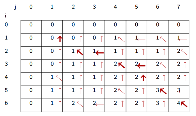
The diagonal arrows in the path correspond to the characters in the LCS. In our case, the LCS has length 4 and it is ABBA.
1
2
3
4
5
6
7
8
9
10
11
12
13
14
15
16
17
18
19
20
21
22
23
24
25
26
27
28
29
30
31

def lcs_length(X, Y, m, n):
    let b[1..m, 1..n] and c[0..m, 0..n] be new tables
    # Initialize 1st row and column to 0
    for i = 1 to m:
        c[i, 0] = 0
    for j = 0 to n:
        c[0, j] = 0
    for i = 1 to m:
        for j = 1 to n:
            if X[i] = Y[j]:
                c[i, j] = c[i-1, j-1] + 1
                b[i, j] = "↖" # up left
            elsif c[i-1, j] >= c[i, j-1]:
                c[i, j] = c[i-1, j]
                b[i, j] = "↑" # up
            else:
                c[i, j] = c[i, j-1]
                b[i, j] = "←" # left
    return b, c


def print_lcs(b, X, i, j):
    if i == 0 or j == 0:
        return
    if b[i, j] == "↖": # up left
        print-lcs(b, X, i-1, j-1)
        print X[i]
    elsif b[i, j] == "↑": # up
        print-lcs(b, X, i-1, j)
    elsif b[i, j] == "←": # left
        print-lcs(b, X, i, j-1)
The runtime of lcs-length is dominated by the two nested loops; runtime is .
The runtime of print-lcs is , where .
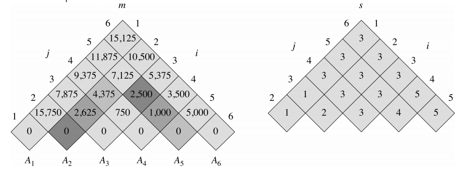
Optimal binary search trees
Given a sequence of keys of distinct keys, sorted so that . We want to build a BST. Some keys are more popular than others: key has probability of being searched for. Our BST should have a minimum expected search cost.
The cost of searching for a key is (we add one because the root is at height 0 but has a cost of 1). The expected search cost would then be:
Optimal BSTs might not have the smallest height, and optimal BSTs might not have highest-probability key at root.
Let denote the expected search cost of an optimal BST of .
With the following inputs:
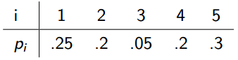
We can fill out the table as follows:
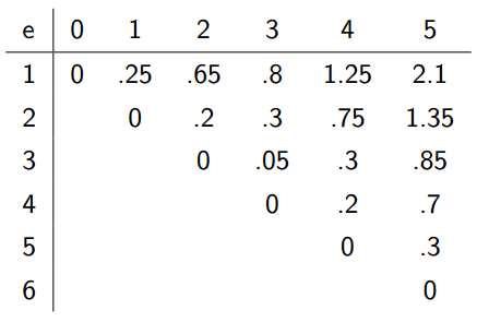
To compute something in this table, we should have already computed everything to the left, and everything below. We can start out by filling out the diagonal, and then filling out the diagonals to its right.
1
2
3
4
5
6
7
8
9
10
11
12
13
14
15
16
17
18

def optimal_bst(p, q, n):
    let e[1..n+1, 0..n] be a new table
    let w[1..n+1, 0..n] be a new table
    let root[1..n, 1..n] be a new table
    for i = 1 to n + 1:
        e[i, i-1] = 0
        w[i, i-1] = 0
    for l = 1 to n:
        for i = 1 to n - l + 1:
            j = i + l - 1
            e[i, j] = infinity
            w[i, j] = w[i, j-1] + p[j]
            for r = i to j:
                t = e[i, r-1] + e[r+1, j] + w[i, j]
                if t < e[i, j]:
                    e[i, j] = t
                    root[i, j] = r
    return (e, root)
-
e[i, j]records the expected search cost of optimal BST of -
r[i, j]records the best root of optimal BST of -
w[i, j]records
The runtime is : there are cells to fill in, most of which take to fill in.
Graphs
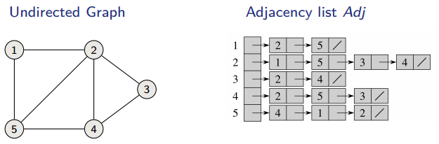
Representation
One way to store a graph is in an adjacency list. Every vertex has a list of vertices to which it is connected. In this representation, every edge is stored twice for undirected graphs, and once for directed graphs.
- Space:
- Time: to list all vertices adjacent to :
- Time: to determine whether
The other way to store this data is in an adjacency matrix. This is a matrix where:
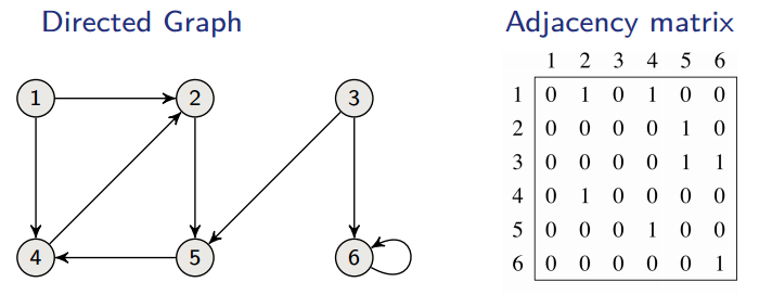
In an undirected graph, this makes for a symmetric matrix. The requirements of this implementation are:
- Space:
- Time: to list all vertices adjacent to :
- Time: to determine whether .
We can extend both representations to include other attributes such as edge weights.
Traversing / Searching a graph
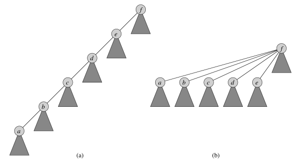
Breadth-First Search (BFS)
- Input: Graph , either directed or undirected and source vertex .
- Output: distance (smallest number of edges) from s to v for all vertices v.
The idea is to:
- Send a wave out from
- First hits all vertices 1 edge from it
- From there, it hits all vertices 2 edges from it…
1
2
3
4
5
6
7
8
9
10
11
12
13
14
15

def BFS(V, E, s):
    # This is Theta(V):
    for each u in V - {s}: # init all distances to infinity
        u.d = infinity
    # This is Theta(1):
    s.d = 0
    Q = Ø
    enqueue(Q, s)
    # This is Theta(E):
    while Q != Ø:
        u = dequeue(Q)
        for each v in G.adj[u]:
            if v.d == infinity:
                v.d = u.d + 1
                enqueue(Q, v)
This is :
- because each vertex is enqueued at most once
- because every vertex is dequeued at most once and we examine the edge only when is dequeued. Therefore, every edge is examined at most once if directed, and at most twice if undirected.
BFS may not reach all vertices. We can save the shortest path tree by keeping track of the edge that discovered the vertex.
Depth-first search (DFS)
- Input: Graph , either directed or undirected
-
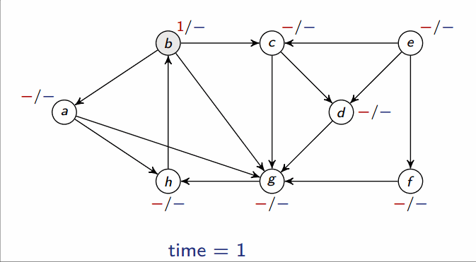
Output: 2 timestamps on each vertex: discovery time
v.dand finishing timev.f
1
2
3
4
5
6
7
8
9
10
11
12
13
14
15
16
17
18

def DFS(G):
    for each u in G.V:
        u.color = WHITE
    time = 0                # global variable
    for each u in G.V:
        if u.color == WHITE:
            DFS_visit(G, u)

def DFS_visit(G, u):
    time = time + 1
    u.d = time
    u.color = GRAY           # discover u
    for each v in G.adj[u]:  # explore (u, v)
        if v.color == WHITE:
            DFS_visit(G, v)
    u.color = BLACK
    time = time + 1
    u.f = time               # finish u
This runs in .
Classification of edges
In DFS of an undirected graph we get only tree and back edges; no forward or back-edges.
Parenthesis theorem
, exactly one of the following holds:
- If v is a descendant of u:
u.d < v.d < v.f < u.f - If u is a descendant of v:
v.d < u.d < u.f < v.f - If neither u nor v are descendants of each other:
[u.d, u.f]and[v.d, v.f]are disjoint (alternatively, we can sayu.d < u.f < v.d < v.forv.d < v.f < u.d < u.f)
White-path theorem
Vertex v is a descendant of u if and only if at time u.d there is a path from u to v consisting of only white vertices (except for u, which has just been colored gray).
Topological sort
- Input: a directed acyclic graph (DAG)
- Output: a linear ordering of vertices such that if , then u appears somewhere before v
1
2
3

def topological sort(G):
    DFS(G) # to compute finishing times v.f forall v
    output vertices in order of decreasing finishing time
Same running time as DFS, .
Topological sort can be useful for ordering dependencies, for instance. Given a dependency graph, it produces a sequential order in which to load them, so that no dependency is loaded before its prerequisite. However, this only works for acyclic dependency graphs; a sequential order cannot arise from cyclic dependencies.
Proof of correctness
We need to show that if then v.f < u.f.
When we explore (u, v), what are the colors of u and v?
- u is gray
- Is v gray too?
- No because then v would be an ancestor of u which implies that there is a back edge so the graph is not acyclic (view lemma below)
- Is v white?
- Then it becomes a descendent of u, and by the parenthesis theorem,
u.d < v.d < v.f < u.f
- Then it becomes a descendent of u, and by the parenthesis theorem,
- Is v black?
- Then v is already finished. Since we are exploring (u, v), we have not yet finished u. Therefore,
v.f < u.f
- Then v is already finished. Since we are exploring (u, v), we have not yet finished u. Therefore,
Lemma: When is a directed graph acyclic?
A directed graph G is acyclic if and only if a DFS of G yields no back edges.
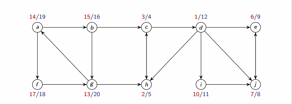
Strongly connected component
A strongly connected component (SCC) of a directed graph is a maximal set of vertices such that .
Below is a depiction of all SCCs on a graph:
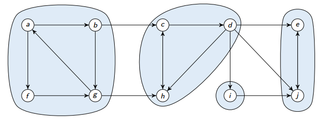
If two SCCs overlap, then they are actually one SCC (and the two parts weren’t really SCCs because they weren’t maximal). Therefore, there cannot be overlap between SCCs.
Lemma
is a directed acyclic graph.
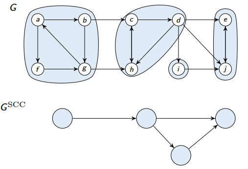
Magic Algorithm
The following algorithm computes SCC in a graph G:
1
2
3
4
5

def SCC(G):
    DFS(G) # to  compute finishing times u.f for all u
    compute G^T
    DFS(G^T) but in the main loop consider vertices in order of decreasing u.f # as computed in first DFS
    Output the vertices in each tree of the DFS forest formed in 2nd DFS as a separate SCC
Where is G with all edges reversed. They have the same SCCs. Using adjacency lists, we can create in time.
Flow Networks
A flow network is a directed graph with weighted edges: each edge has a capacity
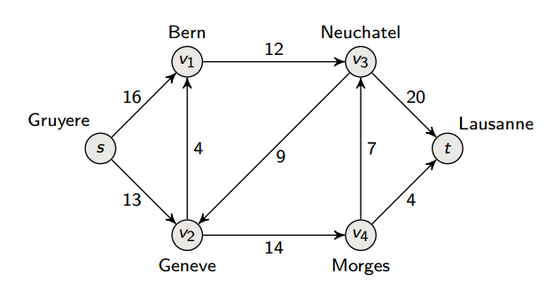
We talk about a source s and a sink t, where the flow goes from s to t.
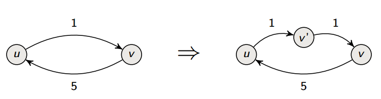
We assume that there are no antiparallel edges, but this is without loss of generality; we make this assumption to simplify our descriptions of our algorithms. In fact, we can just represent antiparallel edges by adding a “temporary” node to split one of the anti-parallel edges in two.
Likewise, vertices can’t have capacities per se, but we can simulate this by replacing a vertex u by vertices uin and uout linked by an edge of capacity cu.
Possible applications include:
- Fire escape plan: exits are sinks, rooms are sources
- Railway networks
- …
We can model the flow as a function . This function satisfies:
Capacity constraint: We do not use more flow than our capacity:
Flow conservation: The flow into u must be equal to the flow out of u
The value of a flow is calculated by measuring at the source; it’s the flow out of the source minus the flow into the source:
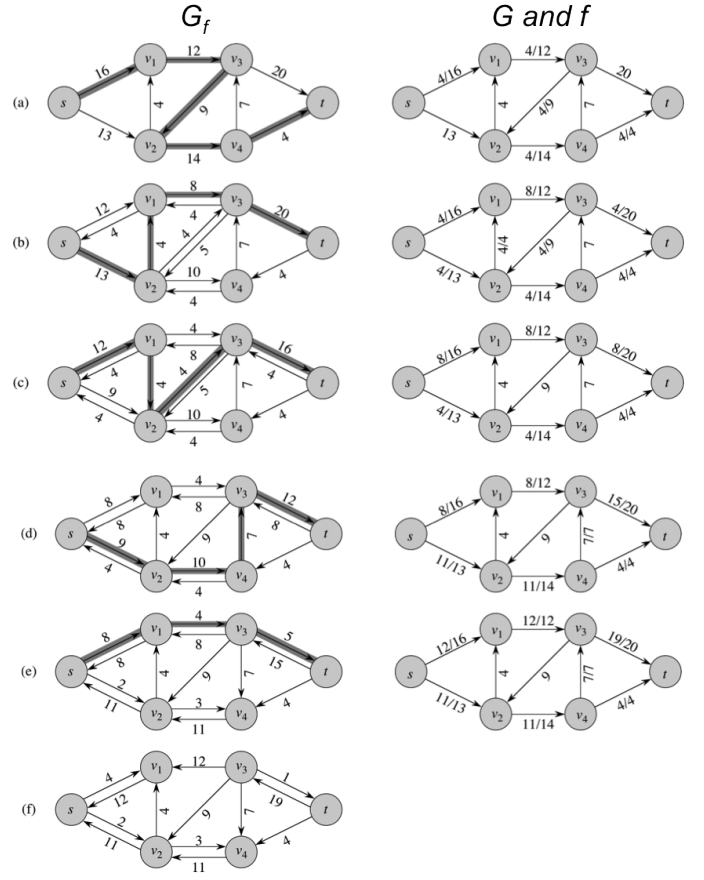
Ford-Fulkerson Method
1
2
3
4
5

def ford_fulkerson_method(G, s, t):
    initialize flow f to 0
    while exists(augmenting path p in residual network Gf):
        augment flow f along p
    return f
As long as there is a path from source to sink, with available capacity on all edges in the path, send flow along one of these paths and then we find another path and so on.
Residual network
The residual network network consists of edges with capacities that represent how we can change the flow on the edges. The residual capacity is:
We can now define the residual network , where:
See the diagram below for more detail:
Cuts in flow networks
A cut of a flow network is a partition of V into two groups of vertices, S and T.
Net flow across a cut
The net flow across the cut (S, T) is the flow leaving S minus the flow entering S.
The net flow across a cut is always equal to the value of the flow, which is the flow out of the source minus the flow into the source. For any cut .
The proof is done simply by induction using flow conservation.
Capacity of a cut
The capacity of a cut (S, T) is:
The flow is at most the capacity of a cut.
Minimum cut
A minimum cut of a network is a cut whose capacity is minimum over all cuts of the network.
The left side of the minimum cut is found by running Ford-Fulkerson and seeing what nodes can be reached from the source in the residual graph; the right side is the rest.
Max-flow min-cut theorem
The max-flow is equal to the capacity of the min-cut.
The proof is important and should be learned for the exam.
Proof of the max-flow min-cut theorem
We’ll prove equivalence between the following:
- has a maximum flow
- has no augmenting path
- for a minimum cut
: Suppose toward contradiction that has an augmenting path p. However, the Ford-Fulkerson method would augment f by p to obtain a flow if increased value which contradicts that f is a maximum flow.
: Let S be the set of nodes reachable from s in a residual network. Every edge flowing out of S in G must be at capacity, otherwise we can reach a node outside S in the residual network.
: Recall that . Therefore, if the value of a flow is equal to the capacity of some cut, then it cannot be further improved.
Time for finding max-flow (or min-cut)
- It takes time to find a a path in the residual network (using for example BFS).
- Each time the flow value is increased by at least 1
- So running time is , where is the value of a max flow.
If capacities are irrational then the Ford-Fulkerson might not terminate. However, if we take the shortest path or fattest path then this will not happen if the capacities are integers (without proof).
| Augmenting path | Number of iterations |
|---|---|
| BFS Shortest path | |
| Fattest path |
Where is the maximum flow value, and the fattest path is the path with largest minimum capacity (the bottleneck).
Bipartite matching
Say we have N students applying for M jobs. Each gets several offers. Is there a way to match all students to jobs?
If we add a source and a sink, give all edges capacity 1, from left to right. If we run Ford-Fulkerson, we get a result.
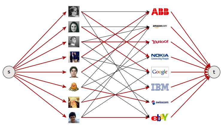
Why does it work?
Every matching defines a flow of value equal to the number of edges in the matching. We put flow 1 on the edges of the matching, and to edges to and from the source and sink. All other edges have 0 flow.
Works because flow conservation is equivalent to: no student is matched more than once, no job is matched more than once.
Edmonds-Kart algorithm
It’s just like Ford-Fulkerson, but we pick the shortest augmenting path (in the sense of the minimal number of edges, found with DFS).
1
2
3
4
5

def edmonds_kart(G):
    while there exists an augmenting path (s, ..., t) in Gf:
        find shortest augmenting path (e.g. using BFS)
        compute bottleneck = min capacity
        augment
The runtime is
Lemma
Let be the shortest path distance from s to u in .
are monotonically non-decreasing throughout the execution of the algorithm.
Proof of runtime
Edmonds-Kart terminates in iterations. An edge (u, v) is said to be critical if its capacity is smallest on the augmenting path.
Every edge in G becomes critical times (a critical edge is removed, but it can reappear later).
Data structures for disjoint sets
- Also known as “union find”
- Maintain collection of disjoint dynamic (changing over time) sets
- Each set is identified by a representative, which is some member of the set. It doesn’t matter which member is the representative, as long as if we ask for the representative twice without modifying the set, we get the same answer both times
We want to support the following operations:
-
make_set(x): Makes a new set and add it to -
union(x, y): If , then- Representative of new set is any member in , often the representative of one of and
- Destroys and (since sets must be disjoint)
-
find(x): Return the representative of the set containingx.
Application: Connected components
1
2
3
4
5
6

def connected_components(G):
    for each vertex v in G.V:
        make_set(v)
    for each edge (u, v) in G.E:
        if find_set(u) != find_set(v):
            union(u, v)
This algorithm runs in in linked-lists with weighted union heuristic, and in forests with union-by-rank and path-compression.
Implementation: Linked List
This is not the fastest implementation, but it certainly is the easiest. Each set is a single linked list represented by a set object that has:
- A pointer to the head of the list (assumed to be the representative)
- A pointer to the tail of the list
Each object in the list has:
- Attributes for the set member (its value for instance)
- A pointer to the set object
- A pointer to the next object
Our operations are now:
-
make_set(x): Create a singleton list in time -
find(x): Follow the pointer back to the list object, and then follow the head pointer to the representative; time .
Union can be implemented in a couple of ways. We can either append y’s list onto the end of x’s list, and update x’s tail pointer to the end.
Otherwise, we can use weighted-union heuristic: we always append the smaller list to the larger list. As a theorem, m operations on n elements takes time.
Implementation: Forest of trees
- One tree per set, where the root is the representative.
- Each node only point to its parent (the root points to itself).
The operations are now:
-
make_set(x): make a single-node tree -
find(x): follow pointers to the root -
union(x, y): make one root a child of another
To implement the union, we can make the root of the smaller tree a child of the root of the larger tree. In a good implementation, we use the rank instead of the size to compare the trees, since measuring the size takes time, and rank is an upper bound on the height of a node anyway. Therefore, a proper implementation would make the root with the smaller rank a child of the root with the larger rank; this is union-by-rank.
find-set can be implemented with path compression, where every node it meets while making its way to the top is made a child of the root; this is path-compression.
find_set(a)Below is one implementation of the operations on this data structure.
1
2
3
4
5
6
7
8
9
10
11
12
13
14
15
16
17
18
19

def make_set(x):
    x.parent = x
    x.rank = 0

def find_set(x):
    if x != x.parent
        x.parent = find_set(x.parent) # path compression
    return x.parent

def union(x, y):
    link(find_set(x), find_set(y)) # path compression here as well

def link(x, y):
    if x.rank > y.rank: # union by rank
        y.parent = x
    else: # if they have the same rank, the 2nd argument becomes parent
        x.parent = y
        if x.rank == y.rank:
            y.rank = y.rank + 1
Minimum Spanning Trees (MST)
A spanning tree of a graph is a set of edges that is:
- Acyclic
- Spanning (connects all vertices)
We want to find the minimum spanning tree of a graph, that is, a spanning tree of minimum total weights.
- Input: an undirected graph G with weight w(u, v) for each edge .
- Output: an MST: a spanning tree of minimum total weights
There are 2 natural greedy algorithms for this.
Prim’s algorithm
Prim’s algorithm is a greedy algorithm. It works by greedily growing the tree T by adding a minimum weight crossing edge with respect to the cut induced by T at each step.
See the slides for a proof.
Implementation
How do we find the minimum crossing edges at every iteration?
We need to check all the outgoing edges of every node, so the running time could be as bad as . But there’s a more clever solution!
- For every node w keep value dist(w) that measures the “distance” of w from the current tree.
- When a new node u is added to the tree, check whether neighbors of u decreases their distance to tree; if so, decrease distance
- Maintain a min-priority queue for the nodes and their distances
1
2
3
4
5
6
7
8
9
10
11
12
13

def prim(G, w, r):
    Q = []
    for each u in G.V:
        u.key = infinity   # set all keys to infinity
        u.pi = Nil
        insert(Q, u)
    decrease_key(Q, r, 0)  # root.key = 0
    while not Q.isEmpty:
        u = extract_min(Q)
        for each v in G.adj[u]:
            if v in Q and w(u, v) < v.key:
                v.pi = u
                decrease_key(Q, v, w(u, v))
When we start every node has the key infinity and our root has key 0, so we pick up the root. Now we need to find the edge with the minimal weight that crosses the cut.
- Initialize Q and first for loop:
-
decrease_keyis - The while loop:
- We run V times
extract_min() - We run E times
decrease_key()
- We run V times
The total runtime is the max of the above, so (which can be made with careful queue implementation).
Kruskal’s algorithm
Start from an empty forest T and greedily maintain forest T which will become an MST at the end. At each step, add the cheapest edge that does not create a cycle.
Implementation
In each iteration, we need to check whether the cheapest edge creates a cycle.
This is the same thing as checking whether its endpoints belong to the same component. Therefore, we can use a disjoint sets (union-find) data structure.
1
2
3
4
5
6
7
8
9
10

def kruskal(G, w):
    A = []
    for each v in G.V:
        make_set(v)
    sort the edges of G.E into nondecreasing order by weight w
    for each (u, v) of the sorted list:
        if find_set(u) != find_set(v): # do they belong to the same CC?
            A = A union {(u, v)} # Add the edge to the MST
            union(u, v) # add the new node to the CC
    return A
- Initialize A:
- First for loop: V times
make_set - Sort E:
- Second for loop: times
find_setsandunions
So this can run in (or, equivalently, since at most); runtime is dominated by the sorting algorithm.
Summary
- Greedy is good (sometimes)
- Prim’s algorithm relies on priority queues for the implementation
- Kruskal’s algorithm uses union-find
Shortest Path Problem
- Input: directed, weighted graph
- Output: a path of minimal weight (there may be multiple solutions)
The weight of a path .
Problem variants
- Single-source: Find shortest paths from source vertex to every vertex
- Single-destination: Find shortest paths to given destination vertex. This can be solved by reversing edge directions in single-source.
- Single pair: Find shortest path from u to v. No algorithm known that is better in worst case than solving single-source.
- All pairs: Find shortest path from u to v for all pairs u, v of vertices. This can be solved with single-pair for each vertex, but better algorithms are knowns
Bellman-Ford algorithm
Bellman-Ford runs in . Unlike Dijkstra, it allows negative edge weights, as long as no negative-weight cycle (a cycle where the weights add up to a negative number) is reachable from the source. The algorithm is easy to implement in distributed settings (e.g. IP routing): each vertex repeatedly asks their neighbors for the best path.
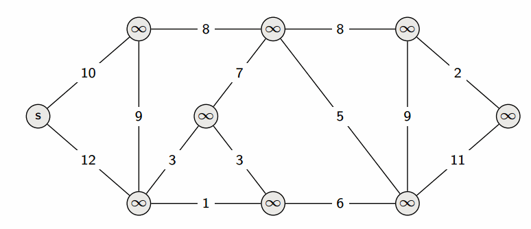
- Input: Directed graph with weighted edges, source s, no negative cycles.
- Ouput: The shortest path from s to t
It starts by trivial initialization, in which the distance of every vertex is set to infinity, and their predecessor is non-existent:
1
2
3
4
5

def init_single_source(G, s):
    for each v in G.V:
        v.distance = infinity
        v.predecessor = Nil
    s.d = 0
Bellman-Ford updates shortest-path estimates iteratively by using relax:
1
2
3
4

def relax(u, v, w):
    if v.distance > u.distance + w(u, v): # if our attempt improves the distance
        v.distance = u.distance + w(u, v)
        v.predecessor = u
This function reduces the distance of v if it is possible to reach it in a shorter path thanks to the (u, v) edge. It runs in .
The entire algorithm is then:
1
2
3
4
5
6
7
8
9
10
11
12

def bellman_ford(G, w, s):
    init_single_source(G, s)
    for i = 1 to |G.V| - 1:
        for each edge (u, v) in G.E:
            relax(u, v, w)
    # Optional: detecting negative cycles
    # Essentially we're just checking whether relax()
    # would change anything on an additional iteration
    for each edge (u, v) in G.E:
        if v.distance > u.distance + w(u, v):
            return False # there is a negative cycle
    return True # there are no negative cycles
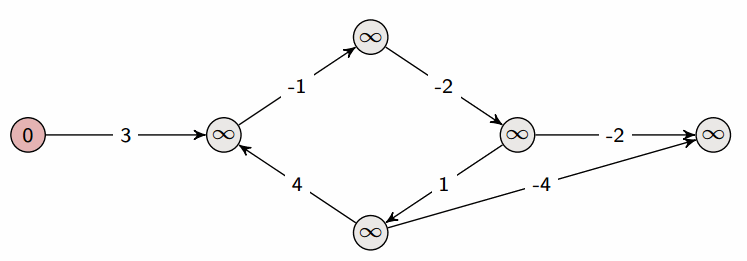
A property of Bellman-Ford:
- After one iteration, we have found all shortest paths that are one edge long
- After two iterations, we have found all shortest paths that are two edges long
- After three iterations, we have found all shortest paths that are three edges long
- …
Let’s assume that the longest shortest path (in terms of number of edges) is from source s to vertex t. Let’s assume that there are n vertices in total; then the shortest path from s to t can at most be n-1 edges long, which is why we terminate at n-1 iterations in the above pseudocode.
Indeed, if there are no negative cycles, Bellman-Ford returns the correct answer after n-1 iterations. But we may in reality already be done before the n-1st iteration. If the longest shortest path (in terms of number of edges) is m edges long, then the mth iteration will produce the final result. The algorithm has no way of knowing the value of m, but what it could do is run an m+1st iteration and see if any distances change; if not, then it is done.
At any iteration, if Bellman-Ford doesn’t change any vertex distances, then it is done (it won’t change anything after this point anyway).
Detecting negative cycles
There is no negative cycle reachable from the source if and only if no distances change when we run one more (nth) iteration of Bellman-Ford.
Dijkstra’s algorithm
- This algorithm only works when all weights are nonnegative.
- It’s greedy, and faster than Bellman-Ford.
- It’s very similar to Prim’s algorithm; could also be described as a weighted version of BFS.
We start with a Source , and greedily grow S. At each step, we add to S the vertex that is closest to S (where distance is defined u.d + w(u, v)).
This creates the shortest-path tree: we can give the shortest path between the source and any vertex in the tree.
Since Dijkstra’s algorithm is greedy (it doesn’t have to consider all edges, only the ones in the immediate vicinity), it is more efficient. Using a binary heap, we can run in (though a more careful implementation can optimize it to ).
1
2
3
4
5
6
7
8
9

def dijkstra(G, w, s):
    init_single_source(G, s)
    S = []
    Q = G.V   # insert all vertices into Q
    while Q != []:
        u = extract_min(Q)
        S = S union {u}
        for each vertex v in G.Adj[u]:
            relax(u, v, w)
Probabilistic analysis and randomized algorithms
Motivation
- Worst case does not usually happen
- Average case analysis
- Amortized analysis
- Randomization sometimes helps avoid worst-case and attacks by evil users
- Choosing the pivot in quick-sort at random
- Randomization necessary in cryptography
- Can we get randomness?
- How to extract randomness (extractors)
- Longer “random behaving” strings from small seed (pseudorandom generators)
Probabilistic Analysis: The Hiring Problem
A basketball team wants to hire a new player. The taller the better. Each candidate that is taller than the current tallest is hired. How many players did we (temporarily) hire?
1
2
3
4
5
6

def hire_player(n):
    best = 0
    for i = 1 to n:
        if candidate i is taller than best candidate so far:
            best = i
            hire i
Worst-case scenario is that the candidates come in sorted order, from lowest to tallest; in this case we hire n players.
What is the expected number of hires we make over all the permutations of the candidates?
There are permutations, each equally likely. The expectation is the sum of hires in each permutation divided by :
For 5 players, we have 120 terms, but for 10 we have 3 628 800… We need to find a better way of calculating this than pure brute force.
Given a sample space and an event A, we define the indicator random variable:
Lemma
For an event A, let . Then
Proof
Multiple Coin Flips
What about multiple coin flips? We want to determine the expected number of heads when we flip n coins. Let be a random variable for the number of heads in n flips. We could calculate:
… but that is cumbersome. Instead, we can use indicator variables.
For , define . Then:
By linearity of expectation (which holds even if X and Y are independent), i.e. that , we have:
For n coin flips, the above yields .
Solving the Hiring Problem
Back to our hiring problem:
Therefore, the number of candidates we can expect to hire is:
This is the harmonic number, which is .
The probability of hiring one candidate is (this is the probability of the first being the tallest), while the probability of hiring all candidates is (which is the probability of the exact permutation where all candidates come in decreasing sorted order).
Bonus trivia
Given a function RANDOM that return 1 with probability and 0 with probability .
Birthday Lemma
If then the probability that a function chosen uniformly at random is injective is at most .
Note that this is a weaker statement than finding the q and m for which f is 50% likely to be injective. The real probability of a such function being injective is , as in the proof below (plugging in shows that in a group of 23, there’s a 50% chance of two people having the same birthday).
Proof
Let . The probability that the function is injective is:
Since we have that this is less than:
Which itself is less than ½ if:
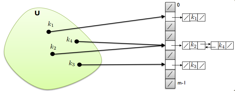
Hash functions and tables
We want to design a computer system for a library, where we can:
- Insert a new book
- Delete book
- Search book
- All operations in (expected) constant time
There are multiple approaches to this; let’s start with a very naive one: a direct-address table, in which we save an array/table T with a position for each possible book (for every possible ISBN).
This is terribly inefficient; sure, the running time of each of the above operations is , but it takes space , where U is the size of the universe.
Hash tables
Instead, let’s use hash tables. Their running time is the same (constant, in average case), but their space requirement is , the size of the key space (instead of the universe).
In hash tables an element with key k is stored in slot h(k). is called the hash function.
A good hash function is efficiently computable, should distribute keys uniformly (seemingly at random over our sample space, though the output should of course be deterministic, the same every time we run the function). This is the principle of simple uniform hashing:
The hashing function h hashes a new key equally likely to any of the m slots, independently of where any other key has hashed to
Collisions
When two items with keys ki and kj have h(ki) = h(kj), we have a collision. How big of a table do we need to avoid collisions with high probability? This is the same problem as the Birthday Lemma. It says that for h to be injective with good probability (meaning that the expected number of collisions is lower than 1) then we need .
This means that if a library has books then it needs an array of size (at least).
Even then, we can’t avoid collisions, but we can still deal with them. We can place all elements that hash to the same slot into the same doubly linked list.
1
2
3
4
5
6
7
8
9

def chained_hash_search(T, k):
    search for an element with key k in list T[h(k)]
    # (this list will often only contain 1 element)

def chained_hash_insert(T, x):
    insert x at the head of list T[h(x.key)]

def chained_hash_delete(T, x):
    delete x in the list T[h(x.key)]
See linked lists for details on how to do operations on the lists.
Running times
-
Insert: -
Delete: -
Search: Expected (if good hash function)
Insertion and deletion are , and the space requirement is .
The worst case is that all n elements are hashed to the same slot, in which case search takes , since we’re searching through a linked list. But this is exceedingly rare with a correct m and n (we cannot avoid collisions without having ).
Let the following be a theorem for running time of search: a search takes expected time , where is the expected length of the list.
See the slides for extended proof!
If we choose the size of our hash table to be proportional to the number of elements stored, we have . Insertion, deletion are then in constant time.
Examples of Hash Functions
- Division method: , where m often selected to be a prime not too close to a power of 2
- Multiplicative method: . Knut suggests chosing .
Quick Sort
We recursively select an element at random, the pivot, and split the list into two sublist; the smaller or equal elements to the left, the larger ones to the right. When we only have single elements left, we can combine them with the pivot in the middle.
This is a simple divide-and-conquer algorithm. The divide step looks like this:
1
2
3
4
5
6
7
8
9

def partition(A, p, r):
    x = A[r] # pivot = last element
    i = p - 1 # i is the separator between left and right
    for j = p to r-1: # iterate over all elements
        if A[j] <= x:
            i = i + 1
            swap A[i] and A[j] # if it needs to go left, set it to
    swap A[i+1] and A[r]
    return i+1 # pivot's new index
See this visualization for a better idea of how this operates.
The running time is for an array of length n; it’s proportional to the number of comparisons we use (the number of times that line 5 is run).
The loop invariant is:
- All entries in
A[p..i]are pivot - All entries in
A[i+1 .. j-1]are pivot -
A[r]is the pivot
The algorithm uses the above like so:
1
2
3
4
5

def quicksort(A, p, r):
    if p < r:
        q = partition(A, p, r)
        quicksort(A, p, q-1) # to the left
        quicksort(A, q+1, r) # to the right
Quicksort runs in if the split is balanced (two equal halves), that is, if we’ve chosen a good pivot. In this case we have our favorite recurrence:
Which indeed is .
But what if we choose a bad pivot every time? We would just have elements to the left of the pivot, and it would run in . But this is very unlikely.
If we select the pivot at random, the algorithm will perform well on any input. Therefore, as a small modification to the partitioning algorithm, we should select a random number in the list instead of the last number.
Total running time is proportional to . We can calculate this by using a random indicator variable:
Note: two numbers are only compared when one is the pivot; therefore, no nunmbers are compared to each other twice (we could also say that two numbers are compared at most once). The total number of comparisons formed by the algorithm is therefore:
The expectancy is thus:
Using linearity of expectation, this is equal to:
- If a pivot such that is chosen then and will never be compared at any later time.
- If either or is chosen before any other element of then it will compared to all other elements of .
- The probability that is compared to is the probability that either or is the element first chosen
- There are elements and pivots chosen at random, independently. Thus the probability that any one of them is the first chosen one is
Therefore:
To wrap it up:
Quicksort is .
Why always n log n?
Let’s look at all the sorting algorithms we’ve looked at or just mentioned during the course:
- Quick Sort
- Merge sort
- Heap sort
- Bubble sort
- Insertion sort
All algorithms we have seen so far have a running time based on the number of comparisons (). Let’s try to analyze the number of comparisons to give an absolute lower bound on sorting algorithms; we’ll find out that it is impossible to do better than .
We need to even examine the inputs. If we look at the comparisons we need no make, we can represent them as a decision tree:
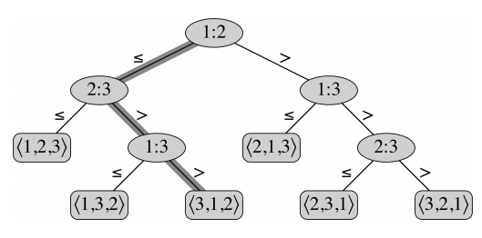
There are leaves in the decision tree (this is the number of output permutations), and its height is . Therefore, if we have an algorithm that takes all its information from comparisons (comparison sorting) gives us a decision tree, and cannot run in better time than . In that sense, merge-sort, heapsort and quicksort are optimal.
Linear time sorting
Also known as non-comparison sort.
-
Input:
A[1..n], where for . ArrayAand valuesnandkare given as parameters -
Output:
B[1..n]sorted
1
2
3
4
5
6
7
8
9
10
11

def counting_sort(A, B, n, k):
    let C[0..k] be a new array
    for i = 0 to k: # initialize C[i] to 0
        C[i] = 0
    for j = 1 to n: # count elements of A
        C[A[j]] = C[A[j]] + 1
    for i = 1 to k: # number of elements with value at most i
        C[i] = C[i] + C[i - 1]
    for j = n downto 1:
        B[C[A[j]]] = A[j]
        C[A[j]] = C[A[j]] - 1 # decrement number of el <= j
The for-loops run in respectively, so runtime is .
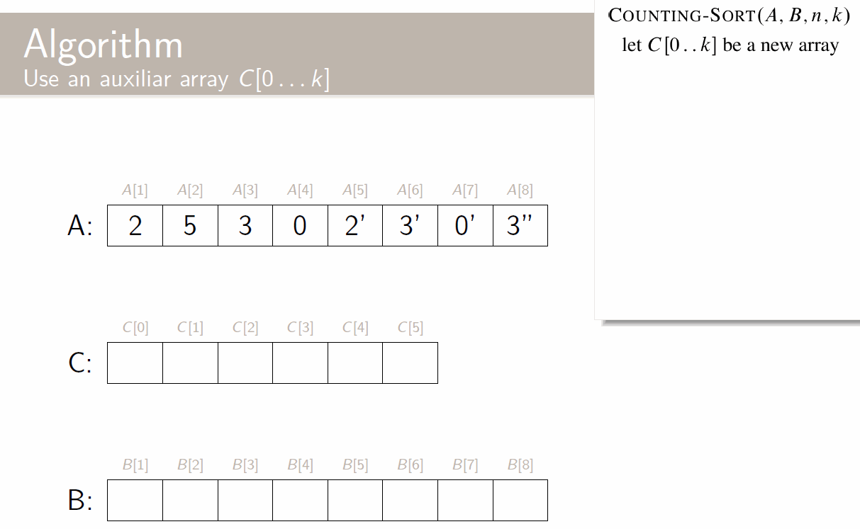
How big a k is practical?
- 32-bit values? No
- 16-bit values? Probably not
- 8-bit values? Maybe depending on n (if it’s big then yes)
- 4-bit values? Probably, unless n is very small (if it’s small then no, comparison sorting is fine)
Review of the course
Growth of functions
- The logs:
- The polynomials:
- The exponentials:
Sorting
- Insertion sort: Put the numers in their correct order one at a time. , worst case occurs when the input is in reverse sorted order
-
Merge sort: A divide and conquer algorithm. The merge works by having two stacks of cards, adding a sentinel at the bottom, and then repeatedly just taking the smallest of the two.
- Time to divide:
- Time to combine
- Number of subproblems and their size: 2 subproblems of size .
- Recurrence: