CS-443 Machine Learning

September 18, 2018

The course follows a few books:

Christopher Bishop, Pattern Recognition and Machine Learning
Kevin Patrick Murphy, Machine Learning: a Probabilistic Perspective
Michael Nielsen, Neural Networks and Deep Learning

The repository for code labs and lecture notes is on GitHub. A useful website for this course is matrixcalculus.org.

Linear regression
Cost functions
- Properties
- Good cost functions
  - MSE
  - MAE
- Convexity
Optimization
Least squares
Maximum likelihood
Overfitting and underfitting
Regularization
- $L_{2}$ -Regularization: Ridge Regression
  - Ridge regression
  - Ridge regression to fight ill-conditioning
- $L_{1}$ -Regularization: The Lasso
Model selection
Classification
Logistic regression
Generalized Linear Models
Nearest neighbor classifiers and the curse of dimensionality
- K Nearest Neighbor (KNN)
- Analysis
Support Vector Machines
Unsupervised learning
Matrix Factorization
SVD and PCA
Neural Networks
Bayes Nets

In this course, we’ll always denote the dataset as a $N \times D$ matrix $X$ , where $N$ is the data size and $D$ is the dimensionality, or the number of features. We’ll always use subscript $n$ for data point, and $d$ for feature. The labels, if any, are denoted in a $y$ vector, and the weights are denoted by $w$ :

w = ⎡ ⎢ ⎢ ⎢ ⎢ ⎣ \begin{matrix} w_{1} w_{2} ⋮ w_{N} \end{matrix} ⎤ ⎥ ⎥ ⎥ ⎥ ⎦, y = ⎡ ⎢ ⎢ ⎢ ⎢ ⎢ ⎣ \begin{matrix} y_{1} y_{2} ⋮ y_{N} \end{matrix} ⎤ ⎥ ⎥ ⎥ ⎥ ⎥ ⎦, X = ⎡ ⎢ ⎢ ⎢ ⎢ ⎢ ⎣ \begin{matrix} x_{11} & x_{12} & \dots & x_{1 D} x_{21} & x_{22} & \dots & x_{2 D} ⋮ & ⋮ & ⋱ & ⋮ x_{N 1} & x_{N 2} & \dots & x_{N D} \end{matrix} ⎤ ⎥ ⎥ ⎥ ⎥ ⎥ ⎦

Vectors are denoted in bold and lowercase (e.g. $y$ or $x_{n}$ ), and matrices are bold and uppercase (e.g. $X$ ). Scalars and functions are in normal font weight¹.

Linear regression

A linear regression is a model that assumes a linear relationship between inputs and the output. We will study three types of methods:

Grid search
Iterative optimization algorithms
Least squares

Simple linear regression

For a single input dimension ( $D = 1$ ), we can use a simple linear regression, which is given by:

y_{n} \approx f (x_{n}) := w_{0} + w_{1} x_{n 1}

$w = (w_{0}, w_{1})$ are the parameters of the model.

Multiple linear regression

If our data has multiple input dimensions, we obtain multivariate linear regression:

y_{n} \approx f (x_{n}) := w_{0} + w_{1} x_{n 1} + \dots + w_{D} x_{w D} = w_{0} + x_{n}^{T} ⎡ ⎢ ⎢ ⎣ \begin{matrix} w_{1} ⋮ w_{D} \end{matrix} ⎤ ⎥ ⎥ ⎦ = {~ x}_{n}^{T} ~ w

👉 If we wanted to be a little more strict, we should write $f_{w} (x_{n})$ , as the model of course also depends on the weights.

The tilde notation means that we have included the offset term $w_{0}$ , also known as the bias:

{~ x}_{n} = ⎡ ⎢ ⎢ ⎢ ⎢ ⎣ \begin{matrix} 1 x_{n 1} ⋮ x_{n D} \end{matrix} ⎤ ⎥ ⎥ ⎥ ⎥ ⎦ \in R^{D + 1}, ~ w = ⎡ ⎢ ⎢ ⎢ ⎢ ⎣ \begin{matrix} w_{0} w_{1} ⋮ w_{D} \end{matrix} ⎤ ⎥ ⎥ ⎥ ⎥ ⎦ \in R^{D + 1}

The $D > N$ problem

If the number of parameters exceeds the number of data examples, we say that the task is under-determined. This can be solved by regularization, which we’ll get to more precisely later.

Cost functions

$x_{n}$ is the data, which we can easily understand where comes from. But how does one find a good $w$ from the data?

A cost function (also called loss function) is used to learn parameters that explain the data well. It quantifies how well our model does by giving errors a score, quantifying penalties for errors. Our goal is to find parameters that minimize the loss functions.

Properties

Desirable properties of cost functions are:

Symmetry around 0: that is, being off by a positive or negative amount is equivalent; what matters is the amplitude of the error, not the sign.
Robustness: penalizes large errors at about the same rate as very large errors. This is a way to make sure that outliers don’t completely dominate our regression.

Good cost functions

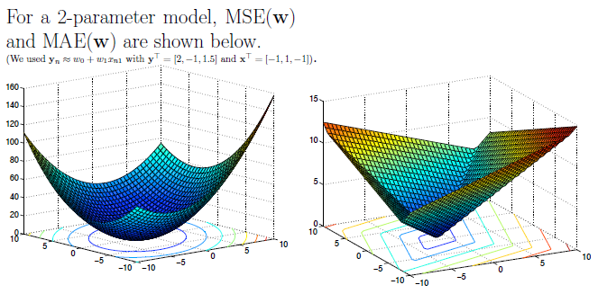
MSE

Probably the most commonly used cost function is Mean Square Error (MSE):

L_{MSE} (w) := \frac{1}{N} N \sum n = 1 {(y_{n} - f (x_{n}))}_{n}^{2}

MSE is symmetrical around 0, but also tends to penalize outliers quite harshly (because it squares error): MSE is not robust. In practice, this is problematic, because outliers occur more often than we’d like to.

Note that we often use MSE with a factor $\frac{1}{2 N}$ instead of $\frac{1}{N}$ . This is because it makes for a cleaner derivative, but we’ll get into that later. Just know that for all intents and purposes, it doesn’t really change anything about the behavior of the models we’ll study.

MAE

When outliers are present, Mean Absolute Error (MAE) tends to fare better:

MAE (w) := \frac{1}{N} N \sum n = 1 | y_{n} - f (x_{n}) |

Instead of squaring, we take the absolute value. This is more robust. Note that MAE isn’t differentiable at 0, but we’ll talk about that later.

There are other cost functions that are even more robust; these are available as additional reading, but are not exam material.

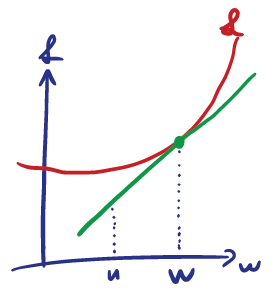
Convexity

A function is convex iff a line joining two points never intersects with the function anywhere else. More strictly defined, a function $f (u)$ with $u \in χ$ is convex if, for any $u, v \in χ$ , and for any $0 \leq λ \leq 1$ , we have:

f (λ u + (1 - λ) v) \leq λ f (u) + (1 - λ) f (v)

A function is strictly convex if the above inequality is strict ( $<$ ). This inequality is known as Jensen’s inequality.

A strictly convex function has a unique global minimum $w^{*}$ . For convex functions, every local minimum is a global minimum. This makes it a desirable property for loss functions, since it means that cost function optimization is guaranteed to find the global minimum.

Linear (and affine) functions are convex, and sums of convex functions are also convex. Therefore, MSE and MAE are convex.

We’ll see another way of characterizing convexity for differentiable functions later in the course.

Optimization

Learning / Estimation / Fitting

Given a cost function (or loss function) $L (w)$ , we wish to find $w^{*}$ which minimizes the cost:

min w L (w), subject to w \in R^{D}

This is what we call learning: learning is simply an optimization problem, and as such, we’ll use an optimization algorithm to solve it – that is, find a good $w$ .

Grid search

This is one of the simplest optimization algorithms, although far from being the most efficient one. It can be described as “try all the values”, a kind of brute-force algorithm; you can think of it as nested for-loops over the individual $w_{i}$ weights.

For instance, if our weights are $w = [\begin{matrix} w_{1} w_{2} \end{matrix}]$ , then we can try, say 4 values for $w_{1}$ , 4 values for $w_{2}$ , for a total of 16 values of $L (w)$ .

But obviously, complexity is exponential $O (a^{D})$ (where $a$ is the number of values to try), which is really bad, especially when we can have $D \approx$ millions of parameters. Additionally, grid search has no guarantees that it’ll find an optimum; it’ll just find the best value we tried.

If grid search sounds bad for optimization, that’s because it is. In practice, it is not used for optimization of parameters, but it is used to tune hyperparameters.

Optimization landscapes

Local minimum

A vector $w^{*}$ is a local minimum of a function $L$ (we’re interested in the minimum of cost functions $L$ , which we denote with $w^{*}$ , as opposed to any other value $w$ , but this obviously holds for any function) if $\exists ϵ > 0$ such that

L (w^{*}) \leq L (w), \forall w : ∥ w - w^{*} ∥ < ϵ

In other words, the local minimum $w^{*}$ is better than all the neighbors in some non-zero radius.

Global minimum

The global minimum $w^{*}$ is defined by getting rid of the radius $ϵ$ and comparing to all other values:

L (w^{*}) \leq L (w), \forall w \in R^{D}

Strict minimum

A minimum is said to be strict if the corresponding equality is strict for $w \neq w^{*}$ , that is, there is only one minimum value.

L (w^{*}) < L (w), \forall w \in R^{D} ∖ {w^{*}}

Smooth (differentiable) optimization

Gradient

A gradient at a given point is the slope of the tangent to the function at that point. It points to the direction of largest increase of the function. By following the gradient (in the opposite direction, because we’re searching for a minimum and not a maximum), we can find the minimum.

Graphs of MSE and MAE

Gradient is defined by:

\nabla L (w) := {[\begin{matrix} \frac{\partial L (w)}{\partial w_{1}} & \frac{\partial L (w)}{\partial w_{2}} & \dots & \frac{\partial L (w)}{\partial w_{D}} \end{matrix}]}^{T}

This is a vector, i.e. $\nabla L (w) \in R^{D}$ . Each dimension $i$ of the vector indicates how fast the cost $L$ changes depending on the weight $w_{i}$ .

Gradient descent

Gradient descent is an iterative algorithm. We start from a candidate $w^{(t)}$ , and iterate.

w^{(t + 1)} := w^{(t)} - γ \nabla L (w^{(t)})

As stated previously, we’re adding the negative gradient to find the minimum, hence the subtraction.

$γ$ is known as the step-size, which is a small value (maybe 0.1). You don’t want to be too aggressive with it, or you might risk overshooting in your descent. In practice, the step-size that makes the learning as fast as possible is often found by trial and error 🤷🏼‍♂️.

As an example, we will take an analytical look at a gradient descent, in order to understand its behavior and components. We will do gradient descent on a 1-parameter model ( $D = 1$ and $w = [w_{0}]$ ), in which we minimize the MSE, which is defined as follows:

L (w_{0}) = \frac{1}{2 N} N \sum n = 1 {(y_{n} - w_{0})}_{n}^{2}

Note that we’re dividing by 2 on top of the regular MSE; it has no impact on finding the minimum, but when we will compute the gradient below, it will conveniently cancel out the $\frac{1}{2}$ .

The gradient of $L (w_{0})$ is:

\begin{matrix} \nabla L (w) & = \frac{\partial}{\partial w_{0}} L (w) = \frac{1}{2 N} N \sum n = 1 - 2 (y_{n} - w_{0}) = w_{0} - ¯ y \end{matrix}

Where $¯ y$ denotes the average of all $y_{n}$ values. And thus, our gradient descent is given by:

\begin{matrix} w_{0}^{(t + 1)} & := w_{0}^{(t)} - γ \nabla L (w) = w_{0}^{(t)} - γ (w_{0}^{(t)} - ¯ y) = (1 - γ) w_{0}^{(t)} + γ ¯ y, where ¯ y := \sum n \frac{y_{n}}{N} \end{matrix}

In this case, we’ve managed to find to this exact problem analytically from gradient descent. This sequence is guaranteed to converge to $w^{*} = ¯ y$ ². This would set the cost function to 0, which is the minimum.

The choice of $γ$ has an influence on the algorithm’s outcome:

If we pick $γ = 1$ , we would get to the optimum in one step
If we pick $γ < 1$ , we would get a little closer in every step, eventually converging to $¯ y$
If we pick $γ > 1$ , we are going to overshoot $¯ y$ . Slightly bigger than 1 (say, 1.5) would still converge; $γ = 2$ would loop infinitely between two points; $γ > 2$ diverges.

Gradient descent for linear MSE

Our linear regression is given by a line $y$ that is a regression for some data $X$ :

y = ⎡ ⎢ ⎢ ⎢ ⎢ ⎢ ⎣ \begin{matrix} y_{1} y_{2} ⋮ y_{N} \end{matrix} ⎤ ⎥ ⎥ ⎥ ⎥ ⎥ ⎦, X = ⎡ ⎢ ⎢ ⎢ ⎢ ⎢ ⎣ \begin{matrix} x_{11} & x_{12} & \dots & x_{1 D} x_{21} & x_{22} & \dots & x_{2 D} ⋮ & ⋮ & ⋱ & ⋮ x_{N 1} & x_{N 2} & \dots & x_{N D} \end{matrix} ⎤ ⎥ ⎥ ⎥ ⎥ ⎥ ⎦

We make predictions by multiplying the data by the weights, so our model is:

f_{w} (x_{n}) = x_{n}^{T} w

We define the error vector by:

e = y - X w, or e_{n} = y_{n} - x_{n}^{T} w

The MSE can then be restated as follows:

L (w) := \frac{1}{2 N} N \sum n = 1 {(y_{n} - x_{n}^{T} w)}_{n}^{2} = \frac{1}{2 N} e^{T} e

And the gradient is, component-wise:

\frac{\partial}{\partial w_{d}} L (w) = - \frac{1}{2 N} N \sum n = 1 2 (y_{n} - x_{n}^{T} w) x_{n d} = - \frac{1}{N} (X_{: d})^{T} e

We’re using column notation $X_{: d}$ to signify column $d$ of the matrix $X$ .

And thus, all in all, our gradient is:

\nabla L (w) = - \frac{1}{N} X^{T} e

To compute this expression, we must compute:

The error $e$ , which takes $2 N \cdot D - 1$ floating point operations (flops) for the matrix-vector multiplication, and $N$ for the subtraction, for a total of $2 N \cdot D + N - 1$ , which is $O (N \cdot D)$
The gradient $\nabla L$ , which costs $2 N \cdot D + D - 1$ , which is $O (N \cdot D)$ .

In total, this process is $O (N \cdot D)$ at every step. This is not too bad, it’s equivalent to reading the data once.

Stochastic gradient descent (SGD)

In ML, most cost functions are formulated as a sum of:

L (w) = \frac{1}{N} N \sum n = 1 L_{n} (w)

In practice, this can be expensive to compute, so the solution is to sample a training point $n \in {1, N}$ uniformly at random, to be able to make the sum go away.

The stochastic gradient descent step is thus:

w^{(t + 1)} := w^{(t)} - γ \nabla L_{n} (w^{(t)})

Why is it allowed to pick just one $n$ instead of the full thing? We won’t give a full proof, but the intuition is that:

E [\nabla L_{n} (w)] = \frac{1}{N} N \sum n = 1 \nabla L_{n} (w) = \nabla (\frac{1}{N} N \sum n = 1 L_{n} (w)) \equiv \nabla L (w)

The gradient of a single n is:

L_{n} (w) = \frac{1}{2} {(y_{n} - x_{n}^{T} w)}_{n}^{2} \nabla L_{n} (w) = (- x_{n}^{T}) (y_{n} - x_{n}^{T} w)

Note that $x_{n}^{T} \in R^{D}$ , and $e_{n} = (y_{n} - x_{n}^{T} w) \in R$ . Computational complexity for this is $O (D)$ .

Mini-batch SGD

But perhaps just picking a single value is too extreme; there is an intermediate version in which we choose a subset $B \subseteq {1, \dots, N}$ instead of a single point.

g := \frac{1}{| B |} \sum n \in B \nabla L_{n} (w^{(t)}) w^{(t + 1)} := w^{(t)} - γ g

Note that if $| B | = N$ then we’re performing a full gradient descent.

The computation of $g$ can be parallelized easily over $| B |$ GPU threads, which is quite common in practice; $| B |$ is thus often dictated by the number of available threads.

Computational complexity is $O (| B | \cdot D)$ .

Non-smooth (non-differentiable) optimization

We’ve defined convexity previously, but we can also use the following alternative characterization of convexity, for differentiable functions:

L (u) \geq L (w) + \nabla L {(w)}^{T} (u - w) \forall u, w ⟺ L convex

Meaning that the function must always lie above its linearization (which is the first-order Taylor expansion) to be convex.

A convex function lies above its linearization

Subgradients

A vector $g \in R^{D}$ such that:

L (u) \geq L (w) + g^{T} (u - w) \forall u

is called a subgradient to the function $L$ at $w$ . The subgradient forms a line that is always below the curve, somewhat like the gradient of a convex function.

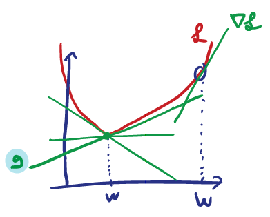
The subgradient lies below the function

This definition is valid even for an arbitrary $L$ that may not be differentiable, and not even necessarily convex.

If the function $L$ is differentiable at $w$ , then the only subgradient at $w$ is $g = \nabla L (w)$ .

Subgradient descent

This is exactly like gradient descent, except for the fact that we use the subgradient $g$ at the current iterate $w^{(t)}$ instead of the gradient:

w^{(t + 1)} := w^{(t)} - γ g

For instance, MAE is not differentiable at 0, so we must use the subgradient.

Let h : R \to R, h (e) := | e | At e, the subgradient g \in \partial h = ⎧ ⎨ ⎩ \begin{matrix} - 1 & if e < 0 [- 1, 1] & if e = 0 1 & if e > 0 \end{matrix}

Here, $\partial h$ is somewhat confusing notation for the set of all possible subgradients at our position.

For linear regressions, the (sub)gradient is easy to compute using the chain rule.

Let $h$ be non-differentiable, $q$ differentiable, and $L (w) = h (q (w))$ . The chain rule tells us that, at $w$ , our subgradient is:

g \in \partial h (q (w)) \cdot \nabla q (w)

Stochastic subgradient descent

This is still commonly abbreviated SGD.

It’s exactly the same, except that $g$ is a subgradient to the randomly selected $L_{n}$ at the current iterate $w^{(t)}$ .

Comparison

	Smooth	Non-smooth
Full gradient descent	Gradient of $L$ Complexity is $O (N \cdot D)$	Subgradient of $L$ Complexity is $O (N \cdot D)$
Stochastic gradient descent	Gradient of $L_{n}$	Subgradient of $L_{n}$

Constrained optimization

Sometimes, optimization problems come posed with an additional constraint.

Convex sets

We’ve seen convexity for functions, but we can also define it for sets. A set $C$ is convex iff the line segment between any two points of $C$ lies in $C$ . That is, $\forall u, v \in C, \forall 0 \leq θ \leq 1$ , we have:

θ u + (1 - θ) v \in C

This means that the line between any two points in the set $C$ must also be fully contained within the set.

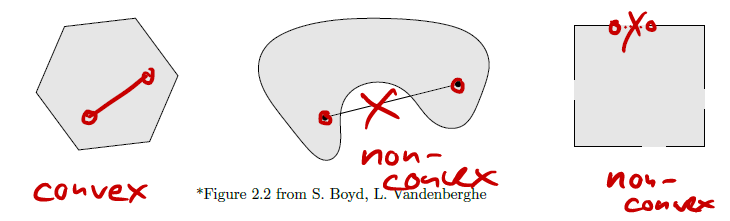
Examples of convex and non-convex sets

A couple of properties of convex sets:

Intersection of convex sets is also convex.
Projections onto convex sets are unique (and often efficient to compute).

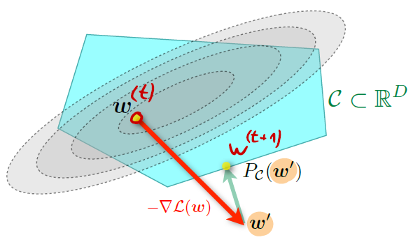
Projected gradient descent

When dealing with constrained problems, we have two options. The first one is to add a projection onto $C$ in every step:

P_{C} (w^{'}) := arg min v \in C ∥ ∥ v - w^{'} ∥ ∥

The rule for gradient descent can thus be updated to become:

w^{(t + 1)} := P_{C} (w^{(t)} - γ \nabla L (w^{(t)}))

This means that at every step, we compute the new $w^{(t + 1)}$ normally, but apply a projection on top of that. In other words, if the regular gradient descent sets our weights outside of the constrained space, we project them back.

Steps of projected SGD — Here, $w^{'}$ is the result of regular SGD, i.e. $w^{'} = w^{(t)} - γ \nabla L (w^{(t)})$

This is the same for stochastic gradient descent, and we have the same convergence properties.

Note that the computational cost of the projection is very important here, since it is performed at every step.

Turning constrained problems into unconstrained problems

If projection as described above is approach A, this is approach B.

We use a penalty function, such as the “brick wall” indicator function below:

I_{C} (w) = {\begin{matrix} 0 & w \in C + \infty & w \notin C \end{matrix}

We could also perhaps use something with a less drastic error value than $+ \infty$ , if we don’t care about the constraint quite as extreme.

Note that this is similar to regularization, which we’ll talk about later.

Now, instead of directly solving ${min}_{w \in C} L (w)$ , we solve for:

min w \in R^{D} L (w) + I_{C} (w)

Implementation issues in gradient methods

Stopping criteria

When $∥ \nabla L (w) ∥$ is zero (or close to zero), we are often close to the optimum.

Optimality

For a convex optimization problem, a necessary condition for optimality is that the gradient is 0 at the optimum:

optimum at w^{*}, L convex ⟹ \nabla L (w^{*}) = 0

For convex functions, if the gradient is 0, then we’re at an optimum:

\nabla L (w^{*}) = 0, L convex ⟹ optimum at w^{*}

This tells us when $w^{*}$ is an optimum, but says nothing about whether it’s a minimum or a maximum. To know about that, we must look at the second derivative, or in the general case where $D > 1$ , the Hessian. The Hessian is the matrix of second derivatives, defined as follows:

H_{i j} = \frac{\partial^{2} L}{\partial w_{i} \partial w_{j}}

If the Hessian of the optimum is positive semi-definite, then it is a minimum (and not a maximum or a saddle point):

H (w^{*}) := \frac{\partial^{2} L (w^{*})}{\partial w \partial w^{T}} positive semidefinite ⟹ w^{*} is a minimum

The Hessian is also related to convexity; it is positive semi-definite on its entire domain (i.e. all its eigenvalues are non-negative) if and only if the function is convex.

H positive semidefinite ⟺ L convex

Step size

If $γ$ is too big, we might diverge (as seen previously). But if it is too small, we might be very slow! Convergence is only guaranteed for $γ < γ_{m i n}$ , which is a value that depends on the problem.

Least squares

Normal equations

In some rare cases, we can take an analytical approach to computing the optimum of the cost function, rather than a computational one; for instance, for linear regression with MSE, as we’ve done previously. These types of equations are sometimes called normal equations. This is one of the most popular methods for data fitting, called least squares.

How do we get these normal equations?

First, we show that the problem is convex. If that is the case, then according to the optimality conditions for convex functions, the point at which the derivative is zero is the optimum:

\nabla L (w^{*}) = 0

This gives us a system of $D$ equations known as the normal equations.

Single parameter linear regression

Let’s try this for a single parameter linear regression (where $D = 1$ ), with MSE as the cost function. We will start by accepting that the cost function is convex in the $w_{0}$ parameter³.

As proven previously, we know that for the single parameter model, the derivative is:

\begin{matrix} \nabla L (w) & = \frac{\partial}{\partial w_{0}} L = \frac{1}{2 N} N \sum n = 1 - 2 (y_{n} - w_{0}) = w_{0} - ¯ y \end{matrix}

This means that the derivative is 0 for $w_{0} = ¯ y$ . This allows us to define our optimum parameter $w^{*}$ as $w^{*} = [\begin{matrix} ¯ y \end{matrix}]$ .

Multiple parameter linear regression

Having done $D = 1$ , let’s look at the general case where $D \geq 1$ . As we know by now, the cost function for linear regression with MSE is:

L (w) := \frac{1}{2 N} N \sum n = 1 {(y_{n} - x_{n}^{T} w)}_{n}^{2} = \frac{1}{2 N} (y - X w)^{T} (y - X w)

Where the matrices are defined as:

y = ⎡ ⎢ ⎢ ⎢ ⎢ ⎢ ⎣ \begin{matrix} y_{1} y_{2} ⋮ y_{N} \end{matrix} ⎤ ⎥ ⎥ ⎥ ⎥ ⎥ ⎦, X = ⎡ ⎢ ⎢ ⎢ ⎢ ⎢ ⎣ \begin{matrix} x_{11} & x_{12} & \dots & x_{1 D} x_{21} & x_{22} & \dots & x_{2 D} ⋮ & ⋮ & ⋱ & ⋮ x_{N 1} & x_{N 2} & \dots & x_{N D} \end{matrix} ⎤ ⎥ ⎥ ⎥ ⎥ ⎥ ⎦

We denote the $i^{th}$ row of $X$ by $x_{i}^{T}$ . Each $x_{i}^{T}$ represents a different data point.

We claim that this cost function is convex in $w$ . We can prove that in any of the following ways:

Simplest way

The cost function is the sum of many convex functions, and is thus also convex.

Directly verify the definition

\forall λ \in [0, 1], \forall w, w^{'}, L (λ w + (1 - λ) w^{'}) - (λ L (w) + (1 - λ) L (w^{'})) \leq 0

The left-hand side of the inequality reduces to:

- \frac{1}{2 N} λ (1 - λ) {∥ ∥ X (w - w^{'}) ∥ ∥}_{2}^{'}

which indeed is $\leq 0$ .

Compute the Hessian

As we’ve seen previously, if the Hessian is positive semidefinite, then the function is convex. For our case, the Hessian is given by:

\frac{1}{N} X^{T} X

This is indeed positive semi-definite, as its eigenvalues are the squares of the eigenvalues of $X$ , and must therefore be positive.

Knowing that the function is convex, we can find the minimum. If we take the gradient of this expression, we get:

\nabla L (w) = - \frac{1}{N} X^{T} (y - X w)

We can set this to 0 to get the normal equations for linear regression, which are:

X^{T} (y - X w) =: X^{T} e = 0

This proves that the normal equations for linear regression are given by $X^{T} e = 0$ .

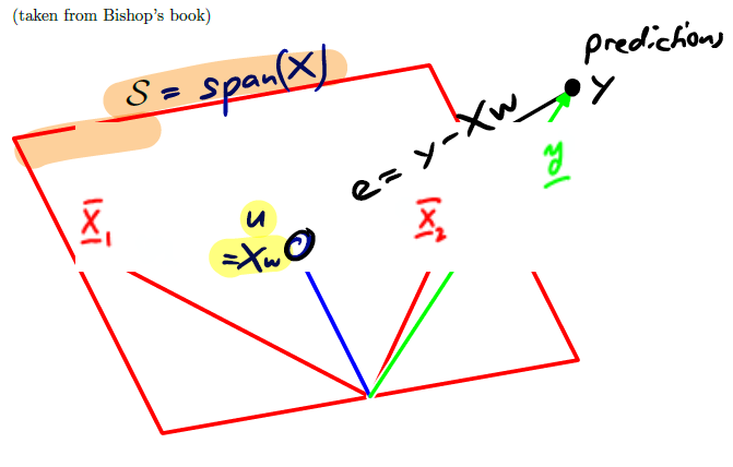
Geometric interpretation

The above definition of normal equations are given by $X^{T} e = 0$ . How can visualize that?

The error is given by:

e := y - X w

By definition, this error vector is orthogonal to all columns of $X$ . Indeed, it tells us how far above or below the span our prediction $y$ is.

The span of $X$ is the space spanned by the columns of $X$ . Every element of the span can be written as $u = X w$ for some choice of $w$ .

For the normal equations, we must pick an optimal $w^{*}$ for which the gradient is 0. Picking an $w^{*}$ is equivalent to picking an optimal $u^{*} = {X w}^{*}$ from the span of $X$ .

But which element of $span (X)$ shall we take, which one is the optimal one? The normal equations tell us that the optimum choice for $u$ , called $u^{*}$ is the element such that $y - u^{*}$ is orthogonal to $span (X)$ .

In other words, we should pick $u^{*}$ to be the projection of $y$ onto $span (X)$ .

Geometric interpretation of the normal equations

Closed form

All we’ve done so far is to solve the same old problem of a matrix equation:

A x = b

But we’ve always done so with a bit of a twist; there may not be an exact value of $x$ satisfying exact equality, but we could find one that gets us as close as possible:

A x \approx b

This is also what least squares does. It attempts to minimize the MSE to get as $A x$ close as possible to $b$ .

In this course, we often denote the data matrix $A$ as $X$ , the weights $x$ as $w$ , and $b$ as $y$ ; in other words, we’re trying to solve:

X w \approx y

In least squares, we multiply this whole equation by $X^{T}$ on the left. We attempt to find $w^{*}$ , the minimal weight that gets us as minimally wrong as possible. In other we’re trying to solve:

(X^{T} X) w \approx X^{T} y

One way to solve this problem would simply be to invert the $A$ matrix, which in our case is $X^{T} X$ :

w^{*} = (X^{T} X)^{- 1} X^{T} y

As such, we can use this model to predict values for unseen data points:

{^y}_{m} := x_{m}^{T} w^{*} = x_{m}^{T} (X^{T} X)^{- 1} X^{T} y

Invertibility and uniqueness

Note that the Gram matrix, defined as $X^{T} X \in R^{D \times D}$ , is invertible if and only if $X$ has full column rank, or in other words, $rank (X) = D$ .

X^{T} X \in R^{D \times D} invertible ⟺ rank (X) = D

Unfortunately, in practice, our data matrix $X \in R^{N \times D}$ is often rank-deficient.

If $D > N$ , we always have $rank (X) < D$ (since column and row rank are the same, which implies that $rank (X) \leq N < D$ ).
If $D \leq N$ , but some of the columns $X_{: d}$ are collinear (or in practice, nearly collinear), then the matrix is ill-conditioned. This leads to numerical issues when solving the linear system.

To know how bad things are, we can compute the condition number, which is the maximum eigenvalue of the Gram matrix, divided by the minimum See course contents of Numerical Methods.

If our data matrix is rank-deficient or ill-conditioned (which is practically always the case), we certainly shouldn’t be inverting it directly! We’ll introduce high numerical errors that falsify our output.

That doesn’t mean we can’t do least squares in practice. We can still use a linear solver. In Python, that means you should use np.linalg.solve, which uses a LU decomposition internally and thus avoids the worst numerical errors. In any case, do not directly invert the matrix as we have done above!

Maximum likelihood

Maximum likelihood offers a second interpretation of least squares, but starting with a probabilistic approach.

Gaussian distribution

A Gaussian random variable in $R$ has mean $μ$ and variance $σ^{2}$ . Its distribution is given by:

N (y ∣ μ, σ^{2}) = \frac{1}{\sqrt{2 π σ^{2}}} exp [- \frac{(y - μ)^{2}}{2 σ^{2}}]

For a Gaussian random vector, we have $y \in R^{N}$ (instead of a single random variable in $R$ ). The vector has mean $μ μ$ and covariance $Σ Σ$ (which is positive semi-definite), and its distribution is given by:

N N (y ∣ μ μ, Σ Σ) = \frac{1}{\sqrt{(2 π)^{D} det (Σ Σ)}} exp [- \frac{1}{2} (y - μ μ)^{T} Σ Σ^{- 1} (y - μ μ)]

As another reminder, two variables $x$ and $y$ are said to be independent when $p (x, y) = p (x) p (y)$ .

A probabilistic model for least squares

We assume that our data is generated by a linear model $x_{n}^{T} w$ , with added Gaussian noise $ϵ_{n}$ :

y_{n} = x_{n}^{T} w + ϵ_{n}

This is often a realistic assumption in practice.

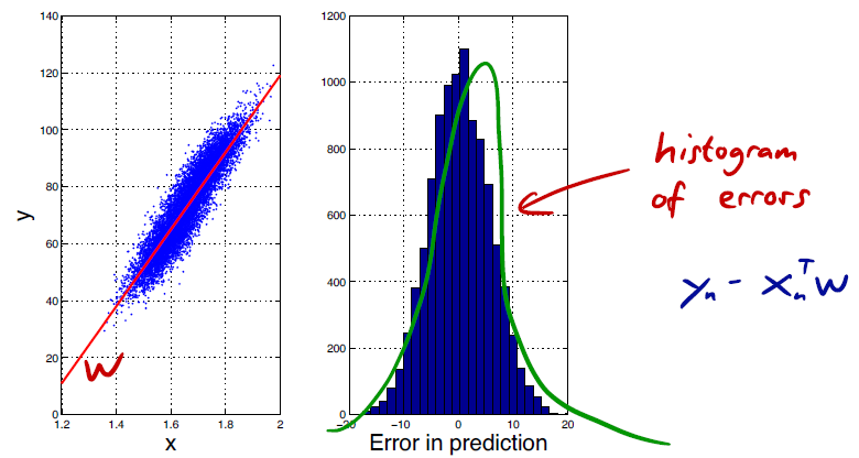
Noise generated by a Gaussian source

The noise is $ϵ_{n} i.i.d. \sim N (y_{n} ∣ μ = 0, σ^{2})$ for each dimension $n$ . In other words, it is centered at 0, has a certain variance, and the error in each dimension is independent of that in other dimensions.

The model $w$ is, as always, unknown. But we can try to do a thought experiment: if we did know the model $w$ the data $X$ , in a system without the noise $ϵ_{n}$ , we would know the labels $y$ with 100% certainty. The only thing that prevents that is the noise $ϵ_{n}$ ; therefore, given the model and data, the probability distribution of seeing a certain $y$ is only given by all the noise sources $ϵ_{n}$ . Since they are generated independently in each dimension, we can take the product of these noise sources.

Therefore, given $N$ samples, the likelihood of the data vector $y = (y_{1}, \dots, y_{n})$ given the model $w$ and the input $X$ is:

p (y ∣ X, w) = N \prod n = 1 p (y_{n} ∣ x_{n}, w) = N \prod n = 1 N (y_{n} ∣ x_{n}^{T} w, σ^{2})

Intuitively, we’d like to maximize this likelihood over the choice of the best model $w$ . The best model is the one that maximizes this likelihood.

Defining cost with log-likelihood

The log-likelihood (LL) is given by:

L_{L L} (w) := log p (y ∣ X, w) = - \frac{1}{2 σ^{2}} N \sum n = 1 {(y_{n} - x_{n}^{T} w)}_{n}^{2} + cnst

Taking the log allows us to get away from the nasty product, and get a nice sum instead. Notice that this definition looks pretty similar to MSE:

L_{MSE} (w) := \frac{1}{N} N \sum n = 1 {(y_{n} - x_{n}^{T} w)}_{n}^{2}

Note that we would like to minimize MSE, but we want the log-likelihood to be as high as possible (intuitively, we can look at the sign to understand that).

Maximum likelihood estimator (MLE)

Maximizing the log-likelihood (and thus the likelihood) will be equivalent to minimizing the MSE; this gives us another way to design cost functions. We can describe the whole process as:

arg min w L_{MSE} (w) = arg max w L_{LL} (w)

The maximum likelihood estimator (MLE) can be understood as finding the model under which the observed data is most likely to have been generated from (probabilistically). This interpretation has some advantages that we discuss below.

Properties of MLE

MLE is a sample approximation to the expected log-likelihood. In other words, if we had an infinite amount of data, MLE would perfectly be equal to the true expected value of the log-likelihood.

L_{L L} (w) \approx E_{p (y, x)} [log p (y ∣ x, w)]

This means that MLE is consistent, i.e. it gives us the correct model assuming we have enough data. This means it converges in probability⁴ to the true value:

w_{MLE} p ⟶ w_{true}

MLE is asymptotically normal, meaning that the difference between the approximation and the true value of the weights converges in distribution⁴ to a normal distribution centered at 0, and with variance $\frac{1}{N}$ times the Fisher information of the true value:

(w_{MLE} - w_{true}) d ⟶ \frac{1}{\sqrt{N}} N (w_{MLE} ∣ 0, F^{- 1} (w_{true}))

Where the Fisher information⁵ is:

F (w) = - E_{p (y)} [\frac{\partial^{2} L}{\partial w \partial w^{T}}]

This sounds amazing, but the catch is that this all is under the assumption that the noise $ϵ$ indeed was generated under a Gaussian model, which may not always be true. We’ll relax this assumption later when we talk about exponential families.

Overfitting and underfitting

Models can be too limited; when we can’t find a function that fits the data well, we say that we are underfitting. But on the other hand, models can also be too rich: in this case, we don’t just model the data, but also the underlying noise. This is called overfitting. Knowing exactly where we are on this spectrum is difficult, since all we have is data, and we don’t know a priori what is signal and what is noise.

Sections 3 and 5 of Pedro Domingos’ paper A Few Useful Things to Know about Machine Learning are a good read on this topic.

Underfitting with linear models

Linear models can very easily underfit; as soon as the data itself is given by anything more complex than a line, fitting a linear model will underfit: the model is too simple for the data, and we’ll have huge errors.

But we can also easily overfit, where our model learns the specificities of the data too intimately. And this happens quite easily with linear combination of high-degree polynomials.

Extended feature vectors

We can actually get high-degree linear combinations of polynomials, but still keep our linear model. Instead of making the model more complex, we simply “augment” the input to become degree $M$ . If the input is one-dimensional, we can add a polynomial basis to the input:

ϕ ϕ (x_{n}) = [\begin{matrix} 1 & x_{n} & x_{n}^{2} & x_{n}^{3} & \dots & x_{n}^{M} \end{matrix}]

Note that this is basically a Vandermonde matrix.

We then fit a linear model to this extended feature vector $ϕ ϕ (x_{n})$ :

y_{n} \approx w_{0} + w_{1} x_{n} + w_{2} x_{n}^{2} + \dots + w_{m} x_{n}^{M} =: ϕ ϕ (x_{n})^{T} w

Here, $w \in R^{M + 1}$ . In other words, there are $M + 1$ parameters in a degree $M$ extended feature vector. One should be careful with this degree; too high may overfit, too low may underfit.

If it is important to distinguish the original input $x$ from the augmented input $ϕ ϕ (x)$ then we will use the $ϕ ϕ (x)$ notation. But often, we can just consider this as a part of the pre-processing, and simply write $x$ as the input, which will save us a lot of notation.

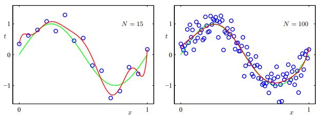
Reducing overfitting

To reduce overfitting, we can chose a less complex model (in the above, we can pick a lower degree $M$ ), but we could also just add more data:

An overfitted model acts more reasonably when we add a bunch of data

Regularization

To prevent overfitting, we can introduce regularization to penalize complex models. This can be applied to any model.

The idea is to not only minimize cost, but also minimize a regularizer:

min w L (w) + Ω (w)

The $Ω$ function is the regularizer, measuring the complexity of the model. We’ll see some good candidates for the regularizer below.

$L_{2}$ -Regularization: Ridge Regression

The most frequently used regularizer is the standard Euclidean norm ( $L_{2}$ -norm):

Ω (w) = λ {∥ w ∥}_{2}^{2}

Where $λ \in R$ . The value of $λ$ will affect the fit; $λ \to 0$ can have overfitting, while $λ \to \infty$ can have underfitting.

The norm is given by:

{∥ w ∥}_{2}^{2} = \sum i w_{i}^{2}

The main effect of this is that large model weights $w_{i}$ will be penalized, while small ones won’t affect our minimization too much.

Ridge regression

Depending on the values we choose for $L$ and $Ω$ , we get into some special cases. For instance, choosing MSE for $L$ is called ridge regression, in which we optimize the following:

min w (\frac{1}{N} N \sum n = 1 {[y_{n} - f (x_{n})]}_{n}^{2} + Ω (w))

Least squares is also a special case of ridge regression, where $λ = 0$

We can find an explicit solution for $w$ in ridge regression by differentiating the cost and regularizer, and setting them to zero:

\begin{matrix} \nabla L (w) & = - \frac{1}{N} X^{T} (y - X w) \nabla Ω (w) & = 2 λ w \end{matrix}

We can now set the full cost to zero, which gives us the result:

w_{ridge}^{*} = (X^{T} X + λ^{'} I)^{- 1} X^{T} y

Where $\frac{λ^{'}}{2 N} = λ$ . Note that for $λ = 0$ , we have the least squares solution.

Ridge regression to fight ill-conditioning

This formulation of $w^{*}$ is quite nice, because adding the identity matrix helps us get something that always is invertible; in cases where we have ill-conditioned matrices, it also means that we can invert with more stability.

We’ll prove that the matrix indeed is invertible. The gist is that the eigenvalues of $(X^{T} X + λ^{'} I)$ are all at least $λ^{'}$ .

To prove it, we’ll write the singular value decomposition (SVD) of $X^{T} X$ as ${U S U}^{T}$ . We then have:

X^{T} X + λ^{'} I = {U S U}^{T} + λ^{'} {U I U}^{T} = U (S + λ^{'} I) U^{T}

The singular value is “lifted” by an amount $λ^{'}$ . There’s an alternative proof in the class notes, but we won’t go into that.

$L_{1}$ -Regularization: The Lasso

We can use a different norm as an alternative measure of complexity. The combination of $L_{1}$ -norm and MSE is known as The Lasso:

min w \frac{1}{2 N} N \sum n = 1 {[y_{n} - f (x_{n})]}_{n}^{2} + λ {∥ w ∥}_{1}

Where the $L_{1}$ -norm is defined as

{∥ w ∥}_{1} := \sum i | w_{i} |

If we draw out a constant value of the $L_{1}$ norm, we get a sort of “ball”. Below, we’ve graphed ${w : {∥ w ∥}_{1} \leq 5}$ .

Graph of the lasso

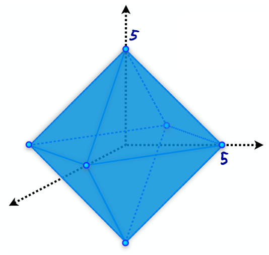
To keep things simple in the following, we’ll just claim that $X^{T} X$ is invertible. We’ll also claim that the following set is an ellipsoid which scales around the origin as we change $α$ :

{w : {∥ y - X w ∥}^{2} = α}

The slides have a formal proof for this, but we won’t get into it.

Note that the above definition of the set corresponds to the set of points with equal loss (which we can assume is MSE, for instance):

{w : L (w) = α}

Under these assumptions, we claim that for $L_{1}$ regularization, the optimum solution will likely be sparse (many zero components) compared to $L_{2}$ regularization.

To prove this, suppose we know the $L_{1}$ norm of the optimum solution. Visualizing that ball, we know that our optimum solution $w^{*}$ will be somewhere on the surface of that ball. We also know that there are ellipsoids, all with the same mean and rotation, describing the equal error surfaces. The optimum solution is where the “smallest” of these ellipsoids just touches the $L_{1}$ ball.

Intersection of the L1 ball and the cost ellipses

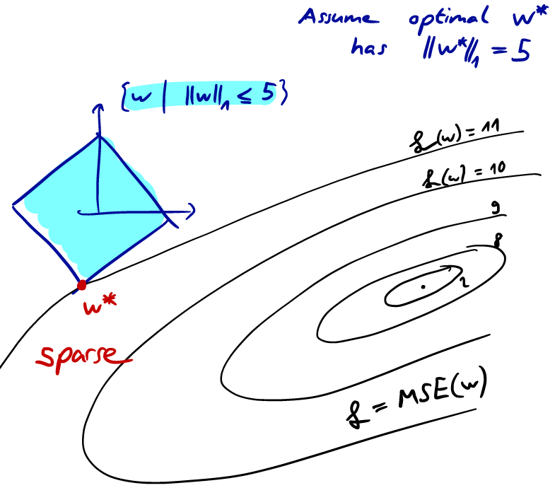
Due to the geometry of this ball this point is more likely to be on one of the “corner” points. In turn, sparsity is desirable, since it leads to a “simple” model.

Model selection

As we’ve seen in ridge regression, we have a regularization parameter $λ > 0$ that can be tuned to reduce overfitting by reducing model complexity. We say that the parameter $λ$ is a hyperparameter.

We’ve also seen ways to enrich model complexity, like polynomial feature expansion, in which the degree $M$ is also a hyperparameter.

We’ll now see how best to choose these hyperparameters; this is called the model selection problem.

Probabilistic setup

We assume that there is an (unknown) underlying distribution $D$ producing the dataset, with range $X \times Y$ . The dataset $S$ we see is produced from samples from $D$ :

S = {(x_{n}, y_{n}) i.i.d \sim D}_{n}^{N}

Based on this, the learning algorithm $A$ choses the “best” model using the dataset $S$ , under the parameters of the algorithm. The resulting prediction function is $f_{s} = A (S)$ . To indicate that $f_{s}$ sometimes depend on hyperparameters, we can write the prediction function as $f_{s, λ}$ .

Training Error vs. Generalization Error

Given a model $f$ , how can we assess if $f$ is any good? We already have the loss function, but its result is highly dependent on the error in the data, not to how good the model is. Instead, we can compute the expected error over all samples chosen according to $D$ .

L_{D} (f) = E_{D} [l (y, f (x))]

Where $l (\cdot, \cdot)$ is our loss function; e.g. for ridge regression, $l (y, f (x)) = \frac{1}{2} (y - f (x))^{2}$ .

The quantity $L_{D} (f)$ has many names, including generalization error (or true/expected error/risk/loss). This is the quantity that we are fundamentally interested in, but we cannot compute it since $D$ is unknown.

What we do know is the data subset⁶ $S$ . It’s therefore natural to compute the equivalent empirical quantity, which is the average loss:

L_{S} (f) = \frac{1}{| S |} \sum (x_{n}, y_{n}) \in S l (y_{n}, f (x_{n}))

But again, we run into trouble. The function $f$ is itself a function of the data $S$ , so what we really do is to compute the quantity:

L_{S} (f_{S}) = \frac{1}{| S |} \sum (x_{n}, y_{n}) \in S l (y_{n}, f_{S} (x_{n}))

$f_{S}$ is the trained model. This is called the training error. Usually, the training error is smaller than the generalization error, because overfitting can happen (even with regularization, because the hyperparameter may still be too low).

Splitting the data

To avoid validating the model on the same data subset we trained it on (which is conducive to overfitting), we can split the data into a training set and a test set (aka validation set), which we call $S_{train}$ and $S_{test}$ , so that $S = S_{train} \oplus S_{test}$ . A typical split could be 80% for training and 20% for testing.

We apply the learning algorithm $A$ on the training set $S_{train}$ , and compute the function $f_{S_{train}}$ . We then compute the error on the test set, which is the test error:

L_{S_{test}} (f_{S_{train}}) = \frac{1}{| S_{test} |} \sum (x_{n}, y_{n}) \in S_{test} l (y_{n}, f_{S_{train}} (x_{n}))

If we have duplicates in our data, then this could be a bit dangerous. Still, in general, this really helps us with the problem of overfitting since $S_{test}$ is a “fresh” sample, which means that we can hope that $L_{S_{test}} (f_{S_{train}})$ defined above is close to the quantity $L_{D} (f_{S_{train}})$ . Indeed, in expectation both are the same:

L_{D} (f_{S_{train}}) = E_{S_{test} \sim D} [L_{S_{test}} (f_{S_{train}})]

The subscript on the expectation means that the expectation is over samples of the test set, and not for a particular test set (which could give a different result due to the randomness of the selection of $S_{test}$ ).

This is a quite nice property, but we paid a price for this. We had to split the data and thus reduce the size of our training data. But we will see that this can be mediated using cross-validation.

Generalization error vs test error

Assume that we have a model $f$ and that our loss function $l (\cdot, \cdot)$ is bounded in $[a, b]$ . We are given a test set $S_{test}$ chosen i.i.d. from the underlying distribution $D$ .

How far apart is the empirical test error from the true generalization error? As we’ve seen above, they are the same in expectation. But we need to worry about the variation, about how far off from the true error we typically are:

We claim that:

\begin{matrix} P [| L_{D} (f) - L_{S_{test}} (f) | \geq \sqrt{\frac{(b - a)^{2} ln (2 / δ)}{2 | S_{test} |}}] \leq δ \\ (loss-bound) \end{matrix}

Where $δ > 0$ is a quality parameter. This gives us an upper bound on how far away our empirical loss is from the true loss.

This bound gives us some nice insights. Error decreases in the size of the test set as $O (1 / \sqrt{| S_{test} |})$ , so the more data points we have, the more confident we can be in the empirical loss being close to the true loss.

We’ll prove $loss-bound$ . We assumed that each sample in the test set is chosen independently. Therefore, given a model $f$ , the associated losses $l (y_{n}, f (x_{n}))$ are also i.i.d. random variables, taking values in $[a, b]$ by assumption. We can call each such loss $Θ_{n}$ :

Θ_{n} = l (y_{n}, f (x_{n}))

This is just a naming alias; since the underlying value is that of the loss function, the expected value of $Θ_{n}$ is simply that of the loss function, which is the true loss:

E [Θ_{n}] = E [l (y_{n}, f (x_{n}))] = L_{D} (f)

The empirical loss on the other hand is equal to the average of $| S_{test} |$ such i.i.d. values.

The formula of $loss-bound$ gives us the probability that empirical loss $L_{S_{test}} (f)$ diverges from the true loss by more than a given constant, which is a classical problem addressed in the following lemma (which we’ll just assert, not prove).

Chernoff Bound: Let $Θ_{1}, \dots, Θ_{N}$ be a sequence of i.i.d random variables with mean $E [Θ]$ and range $[a, b]$ . Then, for any $ϵ > 0$ :

\begin{matrix} P [∣ ∣ ∣ ∣ \frac{1}{N} N \sum n = 1 Θ_{n} - E [Θ] ∣ ∣ ∣ ∣ \geq ϵ] \leq 2 exp (\frac{- 2 N ϵ^{2}}{(b - a)^{2}}) \\ (Chernoff) \end{matrix}

Using $Chernoff$ we can show $loss-bound$ . By setting $δ = 2 exp (\frac{- 2 N ϵ^{2}}{(b - a)^{2}})$ , we find that $ϵ = \sqrt{\frac{(b - a)^{2} ln (2 / δ)}{2 | S_{test} |}}$ as claimed.

Method and criteria for model selection

Grid search on hyperparameters

Our main goal was to look for a way to select the hyperparameters of our model. Given a finite set of values $λ_{k}$ for $k = 1, \dots, K$ of a hyperparameter $λ$ , we can run the learning algorithm $K$ times on the same training set $S_{train}$ , and compute the $K$ prediction functions $f_{S_{train}, λ_{k}}$ . For each such prediction function we compute the test error, and choose the $λ_{k}$ which minimizes the test error.

Grid search on lambda

This is essentially a grid search on $λ$ using the test error function.

Model selection based on test error

How do we know that, for a fixed function $f$ , $L_{S_{test}} (f)$ is a good approximation to $L_{D} (f)$ ? If we’re doing a grid search on hyperparameters to minimize the test error $L_{S_{test}} (f)$ , we may pick a model that obtains a lower test error, but that may increase $| L_{D} (f) - L_{S_{test}} (f) |$ .

We’ll therefore try to see how much the bound increases if we pick a false positive, a model that has lower test error but that actually strays further away from the generalization error.

The answer to this follows the same idea as when we talked about generalization vs test error, but we now assume that we have $K$ models $f_{k}$ for $k = 1, \dots, K$ . We assume again that the loss function is bounded in $[a, b]$ , and that we’re given a test set whose samples are chosen i.i.d. in $D$ .

How far is each of the $K$ (empirical) test errors $L_{S_{test}} (f_{k})$ from the true $L_{D} (f_{k})$ ? As before, we can bound the deviation for all $k$ candidates, by:

P [max k | L_{D} (f_{k}) - L_{S_{test}} (f_{k}) | \geq \sqrt{\frac{(b - a)^{2} ln (2 K / δ)}{2 | S_{test} |}}] \leq δ

A bit of intuition of where this comes from: for a general $K$ , we check the deviations for $K$ independent samples and ask for the probability that for at least one such sample we get a deviation of at least $ϵ$ (this is what the $Chernoff$ bound answers). Then by the union bound this probability is at most $K$ times as large as in the case where we are only concerned with a single instance. Thus the upper bound in Chernoff becomes $2 K exp (\frac{- 2 N ϵ^{2}}{(b - a)^{2}})$ , which gives us $ϵ = \sqrt{\frac{(b - a)^{2} ln (2 K / δ)}{2 | S_{test} |}}$ as above.

As before, this tells us that error decreases in $O (1 / \sqrt{| S_{test} |})$ .

However, now that we test $K$ hyperparameters, our error only goes up by a tiny amount of $\sqrt{ln (K)}$ . This follows from $loss-bound$ , which we proved for the special case of $K = 1$ . So we can reasonably do grid search, knowing that in the worst case, the error will only increase by a tiny amount.

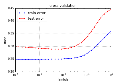
Cross-validation

Splitting the data once into two parts (one for training and one for testing) is not the most efficient way to use the data. Cross-validation is a better way.

K-fold cross-validation is a popular variant. We randomly partition the data into $K$ groups, and train $K$ times. Each time, we use one of the $K$ groups as our test set, and the remaining $K - 1$ groups for training.

To get a common result, we average out the $K$ results. This means we’ll use the average weights to get the average test error over the $K$ folds.

Cross-validation returns an unbiased estimate of the generalization error and its variance.

Bias-Variance decomposition

When we perform model selection, there is an inherent bias–variance trade-off.

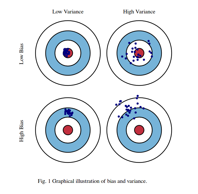
Bullseye representation of bias vs variance — Graphical illustration of bias and variance. Taken from Scott Fortmann-Roe's website

If we were to build the same model over and over again with re-sampled datasets, our predictions would change because of the randomness in the used datasets. Bias tells us how far off from the correct value our predictions are in general, while variance tells us about the variability in predictions for a given point in-between realizations of the models.

For now, we’ll just look at “high-bias & low-variance” models, and “high-variance & low-bias” models.

High-bias & low-variance: the model is too simple. It’s underfit, has a large bias, and and the variance of $L_{D} (f_{S})$ is small (the variations due to the random sample $S$ ).
High-variance & low-bias: the model is too complex. It’s overfit, has a small bias and large variance of $L_{D} (f_{S})$ (the error depends largely on the exact choice of $S$ ; a single addition of a data point is likely to change the prediction function $f_{S}$ considerably)

Consider a linear regression with one-dimensional input and polynomial feature expansion of degree $d$ . The former can be achieved by picking a too low value for $d$ , while the latter by picking $d$ too high. The same principle applies for other parameters, such as ridge regression with hyperparameter $λ$ .

Data generation model

Let’s assume that our data is generated by some arbitrary, unknown function $f$ , and a noise source $ϵ$ with distribution $D_{ϵ}$ (i.i.d. from sample to sample, and independent from the data). We can think of $f$ representing the precise, hypothetical function that perfectly produced the data. We assume that the noise has mean zero (without loss of generality, as a non-zero mean could be encoded into $f$ ).

y = f (x) + ϵ

We assume that $x$ is generated according to some fixed but unknown distribution $D_{x}$ . We’ll be working with square loss $l (y, f (x)) = \frac{1}{2} (y - f (x))^{2}$ . We will denote the joint distribution on pairs $(x, y)$ as $D$ .

\begin{matrix} ϵ & \sim D_{ϵ} x & \sim D_{x} (x, y) & \sim D \end{matrix}

Error Decomposition

As always, we have a training set $S_{train}$ , which consists of $N$ i.i.d. samples from $D$ . Given our learning algorithm $A$ , we compute the prediction function $f_{S_{train}} = A (S_{train})$ . The square loss of a single prediction for a fixed element $x_{0}$ is given by the computation of:

l (y_{0}, f_{S_{train}} (x_{0})) = (y_{0} - f_{S_{train}} (x_{0}))^{2} = (f (x_{0}) + ϵ - f_{S_{train}} (x_{0}))^{2}

Our experiment was to create $S_{train}$ , learn $f_{S_{train}}$ , and then evaluate the performance by computing the square loss for a fixed element $x_{0}$ . If we run this experiment many times, the expected value is written as:

E_{S_{train} \sim D, ϵ \sim D_{ϵ}} [{(f (x_{0}) + ϵ - f_{S_{train}} (x_{0}))}_{0}^{2}]

This expectation is over randomly selected training sets of size $N$ , and over noise sources. We will now show that this expression can be rewritten as a sum of three non-negative terms:

\begin{matrix} E_{S_{train} \sim D, ϵ \sim D_{ϵ}} [{(f (x_{0}) + ϵ - f_{S_{train}} (x_{0}))}_{0}^{2}] (a) = & E_{ϵ \sim D_{ϵ}} [ϵ^{2}] + E_{S_{train} \sim D} [(f (x_{0}) - f_{S_{train}} (x_{0}))^{2}] (b) = & {Var}_{ϵ \sim D_{ϵ}} [ϵ] + E_{S_{train} \sim D} [(f (x_{0}) - f_{S_{train}} (x_{0}))^{2}] (c) = & {Var}_{ϵ \sim D_{ϵ}} [ϵ]      noise variance + {(f (x_{0}) - E_{S_{train}^{'} \sim D} [f_{S_{train}^{'}} (x_{0})])}_{0}^{2}      bias + E_{S_{train} \sim D} ⎡ ⎢ ⎢ ⎢ ⎣ {(E_{S_{train}^{'} \sim D} [f_{S_{train}^{'}} (x_{0})] - f_{S_{train} (x_{0})})}_{S_{train}^{'} \sim D}^{2}      variance ⎤ ⎥ ⎥ ⎥ ⎦ \end{matrix}

Note that here, $S_{train}^{'}$ is a second training set, also sampled from $D$ , that is independent of the training set $S_{train}$ . It has the same expectation, but it is different and thus produces a different trained model $f_{S^{'}}$ .

Step $(a)$ uses $(u + v)^{2} = u^{2} + 2 u v + v^{2}$ as well as linearity of expectation to produce $E [(u + v)^{2}] = E [u^{2}] + 2 E [u v] + E [v^{2}]$ . Note that the $2 u v$ part is zero as the noise $ϵ$ is independent from $S_{train}$ .

Step $(b)$ uses the definition of variance as:

Var (X) = E [(X - E [X])^{2}] = E [X^{2}] - E {[X]}^{2}

Seeing that our noise $ϵ$ has mean zero, we have $E {[ϵ]}^{2} = 0$ and therefore $Var (ϵ) = E [ϵ^{2}]$ .

In step $(c)$ , we add and subtract the constant term $E_{S_{train}^{'} \sim D} [f_{S_{train}^{'}} (x_{0})]$ to the expression like so:

E_{S_{train} \sim D} ⎡ ⎢ ⎢ ⎢ ⎣ {⎛ ⎜ ⎜ ⎝ f (x_{0}) - E_{S_{train}^{'} \sim D} [f_{S_{train}^{'}} (x_{0})]      u + E_{S_{train}^{'} \sim D} [f_{S_{train}^{'}} (x_{0})] - f_{S_{train}} (x_{0})      v ⎞ ⎟ ⎟ ⎠}^{2} ⎤ ⎥ ⎥ ⎥ ⎦

We can then expand the square $(u + v)^{2} = u^{2} + 2 u v + v^{2}$ , where $u^{2}$ becomes the bias, and $v^{2}$ the variance. We can drop the expectation around $u^{2}$ as it is over $S_{train}$ , while $u^{2}$ is only defined in terms of $S_{train}^{'}$ , which is independent from $S_{train}$ . The $2 u v$ part of the expansion is zero, as we show below:

\begin{matrix} 2 \cdot E_{S_{train} \sim D} [(f (x_{0}) - E_{S_{train}^{'} \sim D} [f_{S_{train}^{'}} (x_{0})]) \cdot (E_{S_{train}^{'} \sim D} [f_{S_{train}^{'}} (x_{0})] - f_{S_{train}} (x_{0}))] = 2 \cdot (f (x_{0}) - E_{S_{train}^{'} \sim D} [f_{S_{train}^{'}} (x_{0})]) \cdot E_{S_{train} \sim D} [E_{S_{train}^{'} \sim D} [f_{S_{train}^{'}} (x_{0})] - f_{S_{train}} (x_{0})] = 2 \cdot (f (x_{0}) - E_{S_{train}^{'} \sim D} [f_{S_{train}^{'}} (x_{0})]) \cdot (E_{S_{train}^{'} \sim D} [f_{S_{train}^{'}} (x_{0})] - E_{S_{train} \sim D} [f_{S_{train}} (x_{0})]) = 0 \end{matrix}

In the first step, we can pull $u$ out of the expectation as it is a constant term with regards to $S_{train}$ . The same reasoning applies to $E_{S_{train}^{'} \sim D} [f_{S_{train}^{'}} (x_{0})]$ in the second step. Finally, we get zero in the third step by realizing that:

E_{S_{train}^{'} \sim D} [f_{S_{train}^{'}} (x_{0})] = E_{S_{train} \sim D} [f_{S_{train}} (x_{0})]

Interpretation of the decomposition

Each of the three terms in non-negative, so each of them is a lower bound on the expected loss when we predict the value for the input $x_{0}$ .

When the data contains noise, then that imposes a strict lower bound on the error we can achieve.
The bias term is a non-negative term that tells us how far we are from the true value, in expectation. It’s the square loss between the true value $f (x_{0})$ and the expected prediction $E_{S_{train}^{'} \sim D} [f_{S_{train}^{'}} (x_{0})]$ , where the expectation is over the training sets. As we discussed above, with a simple model we will not find a good fit on average, which means the bias will be large, which adds to the error we observe.
The variance term is the variance of the prediction function. For complex models, small variations in the data set can produce vastly different models, and our prediction will vary widely, which also adds to our total error.

Classification

When we did regression, our data was of the form:

S_{train} = {(x_{n}, y_{n})}_{n}^{N}, x_{n} \in R^{d}, y_{n} \in R

With classification, our prediction is no longer discrete. Now, $y_{n} \in {C_{0}, \dots, C_{K - 1}}$ . If it can only take two values (i.e. $K = 2$ ), then it is called binary classification. If it can take more than two values, it is multi-class classification.

There is no ordering among these classes, so we may sometimes denote these labels as $y \in {0, 1, 2, \dots, K - 1}$ .

If we knew the underlying distribution $D$ , then it would be clear how we could measure the probability of error. We have a correct prediction when $y - f (x) = 0$ , and an incorrect one otherwise, so:

E_{D} [I {y - f (x) \neq 0}] = P (y - f (x) \neq 0)

Where $I$ is an indicator function that returns 1 when the condition is correct, and 0 otherwise. If we don’t know the distribution, we could just take an empirical sum, and use that instead.

A classifier will divide the input space into a collection of regions belonging to each class; the boundaries are called decision boundaries.

Linear classifier

A linear classifier splits the input with a line in 2D, a plane in 3D, or more generally, a hyperplane. But a linear classifier can also classify more complex shapes if we allow for feature augmentation. For instance (in 2D), if we augment the input to degree $M = 2$ and a constant factor, our linear classifier can also detect ellipsoids. So without loss of generality, we’ll simply study linear classifiers and allow feature augmentation, without loss of generality.

Is classification a special case of regression?

From the initial definition of classification, we see that it is a special case of regression, where the output $y$ is restricted to a small discrete set instead of a continuous spectrum.

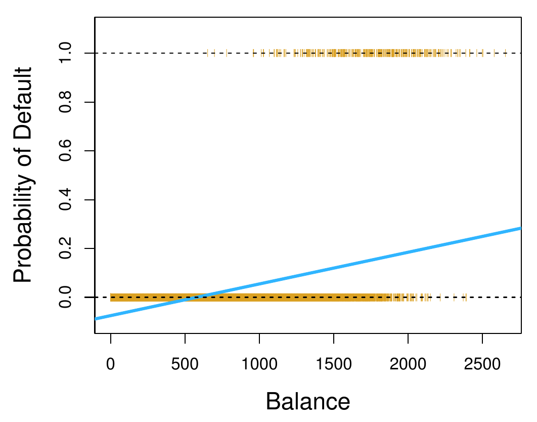
We could construct classification from regression by simply rounding to the nearest $C_{i}$ value. For instance, if we have $y \in {0, 1}$ , we can use (regularized) least-squares to learn a prediction function $f_{S_{train}}$ for this regression problem. We can then convert the regression to a classification by rounding: we decide on $C_{1} = 0$ if $f_{S_{train}} (x) < 0.5$ and $C_{2} = 1$ if $f_{S_{train}} (x) > 0.5$ .

But this is somewhat questionable as an approach. MSE penalizes points that are far away from the result before rounding, even though they would be correct after rounding.

This means that if we have a small loss with MSE, we can guarantee a small classification error (as before), but crucially, the opposite is not true: a regression function can have very high MSE though the classification error is very very small.

It also means that the regression line will likely not be very good. With MSE, the “position” of the line defined by $f_{S_{train}}$ will depend crucially on how many points are in each class, and where the points lie. This is not desirable for classification: instead of minimizing the cost function, we’d like for the fraction of misclassified cases to be small. The mean-squared error turns out to be only loosely related to this.

Example of a regression being skewed by the number of points in each class

So instead of building classification as a special case of regression, let’s take a look at some basic alternative ideas to perform classification.

Nearest neighbor

In some cases it is reasonable to postulate that there is some spatial correlations between points of the same class: inputs that are “close” are also likely to have the same label. Closeness may be measured by Euclidean distance, for instance.

This can be generalized easily: instead of taking the single nearest neighbor, a process very prone to being swayed by outliers, we can take the $k$ nearest neighbors (which we’ll talk about later in the course), or a weighted linear combination of elements in the neighborhood (smoothing kernels, which we won’t talk about).

But this idea fails miserably in high dimensions, where the geometry renders the idea of “closeness” meaningless. High-dimensional space is a very lonely place; in a high-dimensional space, if we grow the area around a point, we’re likely to see no one for a very long time, and then once we get close to the boundaries of the space, 💥, everyone is there at once. This is known as the curse of dimensionality.

The idea also fails when we have too little data, especially in high dimensions, where the closest point may actually be far away and a very bad indicator of the local situation.

Linear decision boundaries

As a starting point, we can assume that decision boundaries are linear (hyperplanes). To keep things simple, we can assume that there is a separating hyperplane, i.e. a hyperplane so that no point in the training set is misclassified.

There may be many such lines, so which one do we pick? This may be a little hand-wavy, but the intuition is the most “robust”, or the one that offers the greatest “margin”: we want to be able to “wiggle” the inputs (by changing the training set) as much as possible while keeping the numbers of misclassifications low. This idea will lead us to support vector machines (SVMs).

But the linear decision boundaries are limited, and in many cases too strong of an assumption. We can augment the feature vector with some non-linear functions, which is what we do with the kernel trick, which we will talk about later. Another option is to use neural networks to find an appropriate non-linear transform of the inputs.

Optimal classification for a known generating model

To find a solution, we can gain some insights if we assume that we know the joint distribution $p (x, y)$ that created the data (where $y$ takes values in a discrete set $y$ ). In practice, we don’t know the model, but this is just a thought experiment. We can assume that the data was generated from a model $(x, y) \sim D$ , where $y = g (x) + ϵ$ , where $ϵ$ is noise.

Given the fact that there is noise, a perfect solution may not always be possible. But if we see an input $x$ , how can we pick an optimal choice $^y (x)$ for this distribution? We want to maximize the probability of guessing the correct label, so we should choose according to the rule:

^y (x) = arg max y \in Y p (y ∣ x)

This is known as the maximum a-posteriori (MAP) criterion, since we maximize the posterior probability (the probability of a class label after having observed the input).

The probability of a correct guess is thus the average over all inputs of the MAP, i.e.:

P (^y (x) = y) = \int p (x) p (^y (x) ∣ x) d x

In practice we of course do not know the joint distribution, but we could use this approach by using the data itself to learn the distribution (perhaps under the assumption that it is Gaussian, and just fitting the $μ$ and $σ$ parameters).

Logistic regression

Recall that we discussed what happens if we look at binary classification as a regression. We also discussed that it is tempting to look at the predicted value as a probability (i.e. if the regression says 0.8, we could interpret it as 80% certainty of $C_{1} = 1$ and 20% probability of $C_{0} = 0$ ). But this leads to problems, as the predicted values may not be in $[0, 1]$ , even largely surpassing these bounds, and this contributes to the error in MSE even though they indicate high certainty.

So the natural idea is to transform the prediction, which can take values in $(- \infty, \infty)$ , into a true probability in $[0, 1]$ . This is done by applying an appropriate function⁷, one of which is the logistic function, or sigmoid function⁸:

σ (z) := \frac{e^{z}}{1 + e^{z}} = \frac{1}{1 + e^{- z}}

How do we use this? Let’s consider binary classification, with labels 0 and 1. Given a training set, we learn a weight vector $w$ . Given a new feature vector $x$ , the probability of the class labels given $x$ are:

\begin{matrix} p (1 ∣ x) & = σ (x^{T} w) p (0 ∣ x) & = 1 - σ (x^{T} w) \end{matrix}

This allows us to predict a certainty, which is a real value and not a label, which is why logistic regression is called regression, even though it is still part of a classification scheme. The second step of the scheme would be to quantize this value to a binary value. For binary classification, we’d pick 0 if the value is less than 0.5, and 1 otherwise.

Training

To train the classifier, the intuition is that we’d like to maximize the likelihood of our weight vector explaining the data:

arg max w p (y, X ∣ w)

We know that maximizing the likelihood is consistent, it gives us the correct model assuming we have enough data. Using the chain rule for probabilities, the probability becomes:

p (y, X ∣ w) = p (X ∣ w) p (y ∣ X, w) = p (X) p (y ∣ X, w)

As we’re trying to get the argmax over the weights, we can discard $p (X)$ as it doesn’t depend on $w$ . Therefore:

arg max w p (y, X ∣ w) = arg max w p (y ∣ X, w)

Using the fact that the samples in the dataset are independent, and given the above formulation of the prior, we can express the maximum likelihood criterion (still for the binary case $K = 2$ )

\begin{matrix} p (y ∣ X, w) & = p (y_{1}, \dots, y_{N} ∣ x_{1}, \dots, x_{N}, w) = N \prod n = 1 p (y_{n} ∣ x_{n}, w) = N \prod n = 1 σ (x_{n}^{T} w)^{y_{n}} (1 - σ (x_{n}^{T} w))^{1 - y_{n}} \end{matrix}

But this product is nasty, so we’ll remove it by taking the log. We also multiply by $- 1$ , which means we also need to be careful about taking the minimum instead of the maximum. The resulting cost function is thus:

\begin{matrix} L (w) & = - N \sum n = 1 [y_{n} log (σ (x_{n}^{T} w)) + (1 - y_{n}) log (1 - σ (x_{n}^{T} w))] = N \sum n = 1 log (1 + exp (x_{n}^{T} w)) - y_{n} x_{n}^{T} w \\ (Log-Likelihood) \end{matrix}

Conditions of optimality

As we discuss above, we’d like to minimize the cost $L (w)$ . Let’s look at the stationary points of our cost function by computing its gradient and setting it to zero.

It just turns out that taking the derivative of the logarithm in the inner part of the sum above gives us the logistic function:

\frac{\partial log (1 + exp (x_{n}^{T} w))}{\partial x_{n}} = σ (x_{n})

Therefore, the whole derivative is:

\begin{matrix} \nabla L (w) & = N \sum n = 1 x_{n} (σ (x_{n}^{T} w) - y_{n}) = X^{T} [σ (X w) - y] \end{matrix}

The matrix $X$ is $N \times N$ ; both $y$ and $w$ are column vectors of length $N$ . Therefore, to simplify notation, we let $σ (X w)$ represent element-wise application of the sigmoid function on the size $N$ vector resulting from $X w$ .

There is no closed-form solution for this, so we’ll discuss how to solve it in an iterative fashion by using gradient descent or the Newton method.

Gradient descent

$Log-Likelihood$ is convex in the weight vector $w$ . We can therefore do gradient descent on this cost function as we’ve always done:

w^{(t + 1)} := w^{(t)} - γ^{(t)} \nabla L (w^{(t)})

Newton’s method

Gradient descent is a first-order method, using only the first derivative of the cost function. We can get a more powerful optimization algorithm using the second derivative. This is based on the idea of Taylor expansions. The 2^nd order Taylor expansion of the cost, around $w^{*}$ , is:

L (w) \approx L {(w^{*})}^{T} (w - w^{*}) + \frac{1}{2} (w - w^{*})^{T} H (w^{*}) (w - w^{*})

Where $H$ denotes the Hessian, the $D \times D$ symmetric matrix with entries:

H_{i, j} = \frac{\partial^{2} L (w)}{\partial w_{i} \partial w_{j}}

Hessian of the cost

Let’s compute this Hessian matrix. We’ve already computed the gradient of the cost function in the section above, where saw that the gradient of a single term is:

x_{n} σ (x_{n}^{T} w) - y_{n}

Each term only depends on $w$ in the $σ (x_{n}^{T} w)$ term. Therefore, the Hessian associated to one term is:

x_{n} (\nabla σ (x_{n}^{T} w))^{T}

Given that the derivative of the sigmoid is $σ^{'} (x) = σ (x) (1 - σ (x))$ , by the chain rule, each term of the sum gives rise to the Hessian:

x_{n} x_{n}^{T} σ (x_{n}^{T} w) (1 - σ (x_{n}^{T} w))

This is the Hessian for a single term; if we sum up over all terms, we get to the following matrix product:

\begin{matrix} H (w) & = N \sum n = 1 \nabla^{2} L_{n} (w) = N \sum n = 1 x_{n} x_{n}^{T}      D \times D σ (x_{n}^{T} w) (1 - σ (x_{n}^{T} w)) = X^{T}      D \times N S    N \times N X    N \times D \end{matrix}

The $S$ matrix is diagonal, with positive entries, which means that the Hessian is positive semi-definite, and therefore that the problem indeed is convex. The entries are:

S_{n, n} = σ (x_{n}^{T} w) (1 - σ (x_{n}^{T} w))

Closed form for Newton’s method

In this model, we’ll assume that the Taylor expansion above denotes the cost function exactly instead of approximately. In other words, we’re assuming strict equality $=$ instead of approximation $\approx$ as above. This is only an assumption; it isn’t strictly true, but it’s a decent approximation. Where does this take minimum value? To know that, let’s set the gradient of the Taylor expansion to zero. This yields:

H (w^{*})^{- 1} \nabla L (w^{*}) = w^{*} - w

If we solve for $w$ , this gives us an iterative algorithm for finding the optimum:

w^{(t + 1)} = w^{(t)} - H {(w^{(t)})}^{- 1} \nabla L (w^{(t)}) γ^{(t)}

The trade-off for the Newton method is that while we need fewer iterations, each of them is more costly. In practice, which one to use depends, but at least we have another option with the Newton method.

Regularized logistic regression

If the data is linearly separable, there is no finite-weight vector. Running the iterative algorithm will make the weights diverge to infinity. To avoid this, we can regularize with a penalty term.

arg min w - N \sum n = 1 log p (y_{n} ∣ x_{n}^{T} w) + \frac{λ}{2} {∥ w ∥}^{2}

Generalized Linear Models

Previously, with least squares, we assumed that our data was of the form:

y = x^{T} w + z, with z \sim N (0, σ^{2})

This is a D-linear model. When talking about generalized linear models, we’re still talking about something linear, but we allow the noise $z$ to be something else than a Gaussian distribution.

Motivation

The motivation for this is that while standard logistic regression only allows for binary outputs⁹, we may want to have something equivalently computationally efficient for, say, $y \in N$ . To do so, we introduce a different class of distributions, called the exponential family, with which we can revisit logistic regression and get other properties.

This will be useful in adding a degree of freedom. Previously, we most often used linear models, in which we model the data as a line, plus zero-mean Gaussian noise. As we saw, this leads to least squares. When the data is more complex than a simple line, we saw that we could augment the features (e.g. with $x^{2}$ , $x^{3}$ ), and still use a linear model. The idea was to augment the feature space $x$ . This gave us an added degree of freedom, and allowed us to use linear models for higher-degree problems.

These linear models predicted the mean of the distribution from which we assumed the data to be sampled. When talking about mean here, we mean what we assume the data to be modeled after, without the noise. In this section, we’ll see how we can use the linear model to predict a different quantity than the mean. This will allow us to add another degree of freedom, and use linear models to get other predictions than just the shape of the data.

We’ve actually already done this, without knowing it. In (binary) logistic regression, the probability of the classes was:

\begin{matrix} p (y = 1 ∣ η) & = σ (η) p (y = 0 ∣ η) & = 1 - σ (η) \end{matrix}

We’re using $η$ as a shorthand for $x^{T} w$ , and will do so in this section. More compactly, we can write this in a single formula:

p (y ∣ η) = \frac{e^{η y}}{1 + e^{η}} = exp [η y - log (1 + e^{η})], y \in {0, 1}

Note that the linear model $x^{T} w$ does not predict the mean, which we’ll denote $μ$ (don’t get confused by this notation; in this section, $μ$ is not a scalar, but represents the “real values” that the data is modeled after, without the noise). Instead, our linear model predicts $η = x^{T} w$ , which is transformed into the mean by using the $σ$ function:

μ = σ (η)

This relation between $μ$ and $σ$ is known as the link function. It is a nonlinear function that makes it possible to use a linear model to predict something else than the mean $μ$ .

Exponential family

In general, the form of a distribution in the exponential family is:

p (y ∣ η η) = h (y) exp [η η^{T} ϕ ϕ (y) - A (η η)]

Let’s take a look at the various components of this distribution:

$ϕ ϕ (y)$ is called a sufficient statistic. It’s usually a vector. Its name stems from the fact that its empirical average is all we need to estimate $η η$
$A (η η)$ is the log-partition function, or the cumulant.

The domain of $y$ can be vary: we could choose $y \in R$ , $y \in {0, 1}$ , $y \in N$ , etc. Depending on this, we may have to do sums or integrals in the following.

We require that the probability be non-negative, so we need to ensure that $h (y) \geq 0$ . Additionally, a probability distribution needs to integrate to 1, so we also require that that:

\int_{y} h (y) exp [η η^{T} ϕ ϕ (y) - A (η η)] d y = 1

This can be rewritten to:

\int_{y} h (y) exp [η η^{T} ϕ ϕ (y)] d y = exp A (η η)

The role of $A (η η)$ is thus only to ensure a proper normalization. To create a member of the exponential family, we can choose the factor $h (y)$ , the vector $ϕ ϕ (y)$ and the parameter $η η$ ; the cumulant $A (η η)$ is then determined for each such choice, and ensures that the expression is properly normalized. From the above, it follows that $A (η η)$ is defined as:

A (η η) = log [\int_{y} h (y) exp [η η^{T} ϕ ϕ (y) - A (η η)] d y]

We exclude the case where the integral is infinite, as we cannot compute a real $A (η η)$ for that case.

Link function

There is a relationship between the mean $μ μ$ and $η η$ using the link function $g$ :

η η = g (μ μ) ⟺ μ μ = g^{- 1} (η η)

The link function is a 1-to-1 transformation from the usual parameters $μ μ$ (e.g. $μ μ = {μ, σ^{2}}$ for Gaussian distributions) to the natural parameters $η η$ (e.g. $η η = {\frac{μ}{σ^{2}}, - \frac{1}{2 σ^{2}}}$ for Gaussian distributions).

For a list of such functions, consult the chapter on Generalized Linear Models in the KPM book.

Example: Bernoulli

The Bernoulli distribution is a member of the exponential family. Its probability density is given by:

\begin{matrix} p (y ∣ μ) & = μ^{y} (1 - μ)^{1 - y}, where μ \in (0, 1) = exp [(log \frac{μ}{1 - μ}) y + log (1 - μ)] = exp [η ϕ (y) - A (η)] \end{matrix}

The parameters are thus:

\begin{matrix} h (y) & = 1 ϕ (y) & = y η & = log \frac{μ}{1 - μ} A (η) & = - log (1 - μ) = log (1 + e^{η}) \end{matrix}

Here, $ϕ (y)$ is a scalar, which means that the family only depends on a single parameter. Note that $η$ and $μ$ are linked:

η = g (μ) = log \frac{μ}{1 - μ} ⟺ μ = g^{- 1} (η) = log \frac{e^{η}}{1 + e^{η}} = σ (η)

The link function is the same sigmoid function we encountered in logistic regression.

Example: Poisson

The Poisson distribution with mean $μ$ is given by:

p (y ∣ μ) = \frac{μ^{y} e^{- μ}}{y!} = \frac{1}{y!} exp [y log (μ) - μ] = h (y) exp [η ϕ (y) - A (η)]

Where the parameters of the exponential family are given by:

\begin{matrix} h (y) & = \frac{1}{y!} ϕ (y) & = y η & = g (μ) = log (μ) A (η) & = μ = g^{- 1} (η) = e^{η} \end{matrix}

Example: Gaussian

Notation for Gaussian distributions can be a little confusing, so we’ll make sure to distinguish the notation of the usual parameter vectors $μ μ$ (in bold), from the parameters themselves, which are the Gaussian mean $μ$ and variance $σ^{2}$ .

The density of a Gaussian $N (μ, σ^{2})$ is:

p (y ∣ μ, σ^{2}) = \frac{1}{\sqrt{2 π σ^{2}}} exp - \frac{(y - μ)^{2}}{2 σ^{2}}, μ \in R, σ \in R^{+}

There are two parameters to choose in a Gaussian, $μ$ and $σ$ , so we can expect something of degree 2 in exponential form. Let’s rewrite the above:

\begin{matrix} p (y ∣ μ, σ^{2}) & = exp ⎡ ⎢ ⎢ ⎢ ⎢ ⎣ - \frac{y^{2}}{2 σ^{2}} + \frac{μ y}{σ^{2}} - \frac{μ^{2}}{2 σ^{2}} - \frac{1}{2} log (2 π σ^{2})      A (η η) ⎤ ⎥ ⎥ ⎥ ⎥ ⎦ = exp [η η^{T} ϕ ϕ (y) - A (η η)] \end{matrix}

Where:

\begin{matrix} h (y) & = 1 ϕ ϕ (y) & = [\begin{matrix} y y^{2} \end{matrix}] η η & = [\begin{matrix} η_{1} η_{2} \end{matrix}] = [\begin{matrix} \frac{μ}{σ^{2}} - \frac{1}{2 σ^{2}} \end{matrix}] A (η η) & = \frac{μ^{2}}{2 σ^{2}} - \frac{1}{2} log (2 π σ^{2}) = \frac{η_{1}^{2}}{4 η_{2}} - \frac{1}{2} log (- η_{2} / π) \end{matrix}

Indeed, this time $ϕ ϕ (y)$ is a vector of dimension 2, which reflects that the distribution depends on 2 parameters. As the formulation of $η η$ shows, we have a 1-to-1 correspondence to $η η = (η_{1}, η_{2})$ and the $(μ, σ^{2})$ parameters:

η_{1} = \frac{μ}{σ^{2}}, η_{2} = - \frac{1}{2 σ^{2}} ⟺ μ = - \frac{η_{1}}{2 η_{2}}, σ^{2} = - \frac{1}{2 η_{2}}

Properties

$A (η η)$ is convex
$\nabla_{η η} A (η η) = E [ϕ ϕ (y)]$
$\nabla_{η η}^{2} A (η η) = E [ϕ ϕ (y)^{T} ϕ ϕ (y)] - E {[ϕ ϕ (y)]}^{T} E [ϕ ϕ (y)]$
$μ μ := E [ϕ ϕ (y)]$

Proofs for the first 3 properties are in the lecture notes. The last property is given without proof.

Application in ML

We use $η_{n} = x_{n}^{T} w$ , or equivalently, $η η = X^{T} w$ .

Maximum Likelihood Parameter Estimation

Assume that we have samples composing our training set, $S_{train} = {(x_{n}, y_{n})}_{n}^{N}$ i.i.d. from some distribution, which we assume is some exponential family. Assume we have picked a model, i.e. that we fixed $h (y)$ and $ϕ ϕ (y)$ , but that $η η$ is unknown. How can we find an optimal $η η$ ?

We said previously that $ϕ ϕ (y)$ is a sufficient statistic, and that we could find $η η$ from its empirical average; this is what we’ll do here. We can use the maximum likelihood principle to find this parameter, meaning that we want to minimize log-likelihood:

\begin{matrix} L_{L L} (η η) & = - log (p (y ∣ η η)) = N \sum n = 1 (- log [h (y_{n})] - η_{n}^{T} ϕ ϕ (y_{n}) + A (η_{n})) \end{matrix}

This is a convex function in $η η$ : the $h (y)$ term does not depend on $η η$ , $η η^{T} ϕ ϕ (y_{n})$ is linear, $A (η η)$ has the property of being convex.

If we assume that we have the link function already, we can get $η η$ by setting the gradient of our exponential family to 0. We also multiply by $\frac{1}{N}$ to get a more convenient form, i.e. with $E [ϕ ϕ (y)]$ instead of $N \cdot E [ϕ ϕ (y)]$ :

\begin{matrix} \frac{1}{N} \nabla L (η η) & = - \frac{1}{N} N \sum n = 1 [ϕ ϕ (y_{n}) - \nabla A (η_{n})] = - \frac{1}{N} (N \sum n = 1 ϕ ϕ (y_{n})) + E [ϕ ϕ (y)] = 0 \end{matrix}

Since $μ μ := E [ϕ ϕ (y)]$ , we get:

μ μ := E [ϕ ϕ (y)] = \frac{1}{N} N \sum n = 1 ϕ ϕ (y_{n})

Therefore, we can get $η η$ by using the link function:

η η = g^{- 1} (μ μ) = g^{- 1} (\frac{1}{N} N \sum n = 1 ϕ ϕ (y_{n}))

With this, we can see the justification for calling $ϕ ϕ (y)$ a sufficient statistic.

Conditions of optimality

If we assume that our samples follow the distribution of an exponential family, we can construct a generalized linear model. As we’ve explained previously, this is a generalization of the model we used for logistic regression.

For such a model, the maximum likelihood problem, as described above, is easy to solve. As we’ve noted above, the cost function is convex, so a greedy, iterative algorithm should work well. Let’s look at the gradient of the cost in terms of $w$ (instead of $η η = x^{T} w$ as previously):

\begin{matrix} L (w) & = - N \sum n = 1 log (h (y_{n})) + x_{n}^{T} w ϕ ϕ (y_{n}) - A (x_{n}^{T} w) \nabla_{w} L (w) & = - N \sum n = 1 x_{n} ϕ ϕ (y_{n}) - \nabla_{w} A (x_{n}^{T} w) \end{matrix}

Let’s recall that the derivative of the cumulant is:

\frac{\partial A (η η)}{\partial η η} = E [ϕ ϕ (y)] = g^{- 1} (η η)

Hence the gradient of the cost function is:

\nabla_{w} L (w) = - N \sum n = 1 x_{n} ϕ ϕ (y_{n}) - x_{n} g^{- 1} (x_{n}^{T} w)

Setting this to zero gives us the condition of optimality. Using matrix notation, we can rewrite this sum as follows:

\nabla_{w} L (w) = X^{T} (g^{- 1} (X w) - ϕ ϕ (y)) = 0

Note that this is a more general form of the formula we had for logistic regression. At this point, seeing that the function is convex, we can use a greedy iterative algorithm like gradient descent to find the minimum.

Nearest neighbor classifiers and the curse of dimensionality

For simplicity, let’s assume that we’re operating in a d-dimensional box, that is, in the domain $χ = [0, 1]^{d}$ . As always, we have a training set $S_{train} = {(x_{n}, y_{n})}$ .

K Nearest Neighbor (KNN)

Given a “fresh” input $x$ , we can make a prediction using ${nbh}_{S_{train}, k} (x)$ . This is a set of the $k$ inputs in the training set that are closest to $x$ .

For the regression problem, we can take the average of the k nearest neighbors:

f (x) = \frac{1}{k} \sum n \in {nbh}_{S_{train}, k} (x) y_{n}

For binary classification, we take the majority element in the $k$ -neighborhood. It’s a good idea to pick $k$ to be odd so that there is a clear winner.

f (x) = maj {y_{n} : n \in {nbh}_{S_{train}, k} (x)}

If we pick a large value of $k$ , then we are smoothing over a large area. Therefore, a large $k$ gives us a simple model, with simpler boundaries, while a small $k$ is a more complex model. In other words, complexity is inversely proportional to $k$ . As we saw when we talked about bias and variance, if we pick a small value of $k$ we can expect a small bias but huge variance. If we pick a large $k$ we can expect large bias but small variance.

Analysis

We’ll analyze the simplest setting, a binary KNN model (that is, there are only two output labels, 0 and 1). Let’s start by simplifying our notation. We’ll introduce the following function:

η (x) = P {y = 1 ∣ x}

This is the conditional probability that the label is 1, given that the input is $x$ . If this probability is to be meaningful at all, we must have some correlation between the “position” x and the associated label; knowing the labels close by must give us some information. This means that we need an assumption on the distribution $D$ :

\begin{matrix} ∣ ∣ η (x) - η (x^{'}) ∣ ∣ \leq c ∥ ∥ x - x^{'} ∥ ∥ \\ (Lipschitz bound) \end{matrix}

On the right-hand side we have Euclidean distance. In other words, we ask that the conditional probability $P {y = 1 ∣ x}$ , denoted by $η (x)$ , be Lipschitz continuous with Lipschitz constant $c$ . We will use this assumption later on to prove a performance bound for our KNN model.

Let’s assume for a moment that we know the actual underlying distribution. This is not something that we actually know in practice, but is useful for deriving a formulation for the optimal model. Knowing the distribution probability distribution, our optimum decision rule is given by the classifier:

f_{*} (x) = I [η (x) > \frac{1}{2}]

The idea of this classifier is that with two labels, we’ll pick the label that is likely to happen more than half of the time. The intuition is that if we were playing heads or tails and knew the probability in advance, we would always pick the option that has probability more than one half, and that is the best strategy we can use. This is known as the Bayes classifier, also called maximum a posteriori (MAP) classifier. It is optimal, in that it has the smallest probability of misclassification of any classifier, namely:

L (f_{*}) = E_{x \sim D} [min {η (x), 1 - η (x)}]

Let’s compare this to the probability of misclassification of the real model:

L (f_{S_{train}, k = 1}) = E [I [f_{S_{train}} (x) \neq y]]

This tells us that the risk (that is, the error probability of our $k = 1$ nearest neighbor classifier) is the above expectation. It’s hard to find a closed form for that expectation, but we can place a bound on it by comparing the ideal, theoretical model to the actual model. We’ll state the following lemma:

\begin{matrix} L (f_{S_{train}}) & \leq 2 L (f_{*}) + c E_{S_{train}, x \sim D} [∥ ∥ x - {nbh}_{S_{train}, 1} (x) ∥ ∥] \leq 2 L (f_{*}) + 4 c \sqrt{d} N^{- \frac{1}{d + 1}} \end{matrix}

Before we see where this comes from, let’s just interpret it. The above gives us a bound on the real classifier, compared to the optimal one. The actual classifier is upper bounded by twice the risk of the optimal classifier (this is good), plus a geometric term reflecting dimensionality (it depends on $d$ : this will cause us some trouble).

This second term of the sum is the average distance of a randomly chosen point to the nearest point in the training set, times the Lipschitz constant $c$ . It intuitively makes sense to incorporate this factor into our bound: if we are basing our prediction on a point that is very close, we’re more likely to be right, and if it’s far away, less so. If we’re in a box of $[0, 1]^{d}$ , then the distance between two corners would be $\sqrt{d}$ (by Pythagoras’ theorem). The term $N^{- \frac{1}{d + 1}}$ indicates that the closest data point may be closer than the opposite corner of the cube: if we have more data, we’ll probably not have to go that far. However, for large dimensions, we need much more data to have something that’ll probably be close.

Let’s prove where this geometric term comes from by considering the cube $[0, 1]^{d}$ , the space of inputs containing $x$ . We can cut this large cube into small cubes of side length $ϵ$ . Consider the small cube containing $x$ . If we are lucky, this small cube also contains a neighboring data point at distance at most $\sqrt{d} ϵ$ (at the opposite corner of the small cube; we use Pythagoras’ theorem as above). However, if we’re less lucky, the closest neighbor may be at the other corner of the big cube, at distance $\sqrt{d}$ . So what is the probability of a point not having a neighbor in its small $ϵ$ cube?

Let’s denote the probability of $x$ landing in a particular box by $P_{i}$ . The chance that none of the N training points are in the box is $(1 - P_{i})^{N}$ . We don’t know the distribution $D$ , so we can’t really express $P_{i}$ in a closed form, but that doesn’t matter, this notation allows us to abstract over that. The rest of the proof is calculus, carefully choosing the right scaling for $ϵ$ in order to get a good bound.

Now, let’s understand where the term $2 L (f_{*})$ comes from. If we flip two coins, $y$ and $y^{'}$ , what is the probability of the outcome being different?

P {y \neq y^{'}} = 2 p (1 - p)

Now, let’s consider two points $x$ and $x^{'}$ , both elements of $[0, 1]^{d}$ . Their labels are $y$ and $y^{'}$ , respectively. The probability of these two labels being different is roughly the same as above (although the probabilities of the two events may not be the same in general):

\begin{matrix} P {y \neq y^{'}} = & η (x) (1 - η (x^{'})) + η (x^{'}) (1 - η (x)) = & 2 η (x) (1 - η (x)) + (2 η (x) - 1) (η (x) - η (x^{'})) \leq & 2 η (x) (1 - η (x)) + (η (x) - η (x^{'})) \leq & 2 η (x) (1 - η (x)) + c ∥ ∥ x - x^{'} ∥ ∥ \end{matrix}

The second to last step uses the fact that $η$ is a probability distribution, so $- 1 \leq 2 η (x) - 1 \leq 1$ . The last step uses the $Lipschitz bound$ .

Therefore, we can confirm the following bound:

P {y \neq y^{'}} \leq 2 η (x) (1 - η x) + c ∥ ∥ x - x^{'} ∥ ∥

But we are still one step away from explaining how we can compare this to the optimal estimator. In the above, we derived a bound for two labels being different. How is this related to our KNN model? The probability of getting a wrong prediction from KNN with $k = 1$ (which we denoted $E_{S_{train}} [L (f_{S_{train}})]$ ) is the probability of the predicted label being different from the solution label.

We get to our lemma by the following reasoning:

2 η (x) (1 - η x) \leq 2 min {η (x), 1 - η (x)} = 2 L (f_{*})

Additionally, the average of the term $c ∥ x - x^{'} ∥$ is $c E_{S_{train}, x \sim D} [∥ ∥ x - {nbh}_{S_{train}, 1} (x) ∥ ∥]$

If we had assumed that it was a ball instead of a cube, we would’ve gotten slightly different results. But that’s besides the point: the main insight from this is that it depends on the dimension, and that for low dimensions at least, we still have a fairly good classifier. But finding a closest neighbor in high dimension can quickly become meaningless.

Support Vector Machines

Definition

Let’s re-consider binary classification. In the following it will be more convenient to consider $y_{n} \in {\pm 1}$ . This is equivalent to what we’ve done previously, under the mapping $0 \mapsto - 1$ and $1 \mapsto 1$ . Note that this mapping can be done continuously in the range $[0, 1] \mapsto [- 1, 1]$ by computing ${~ y}_{n} = 2 y_{n} - 1$ , and back with $y_{n} = \frac{1}{2} ({~ y}_{n} + 1)$ .

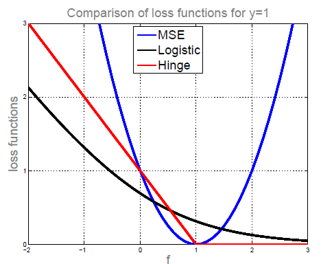
Previously, we used MSE or logistic loss. MSE is symmetric, so something being positive or negative is punished at an equal rate. With logistic regression, we always have a loss, but its value is asymmetric, shrinking the further we go right.

If we instead use hinge loss (as defined below), with an additional regularization term, we get Support Vector Machines (SVM).

Hinge (z, y) = [1 - y z]_{+} = max {0, 1 - y z}

Here, we use $z$ as shorthand for $x^{T} w$ . The function multiplies the prediction with the actual label, which produces a positive result if they are of the same sign, and a negative result if they have different signs (this is why we wanted our labels in ${\pm 1}$ ). When the prediction is correct and above one, $1 - y z$ becomes negative, and hinge loss returns 0. This makes hinge loss a linear function when predictions are incorrect or below one; it does not punish correct predictions above one, which pushes us to give predictions that we can be very confident about (above one).

Graph of hinge loss, MSE and logistic

SVMs correspond to the following optimization problem:

min w N \sum n = 1 {[1 - y_{n} x_{n}^{T} w]}_{+} + \frac{λ}{2} {∥ w ∥}^{2}

What does this optimization problem correspond to, intuitively?

Margin of a dataset

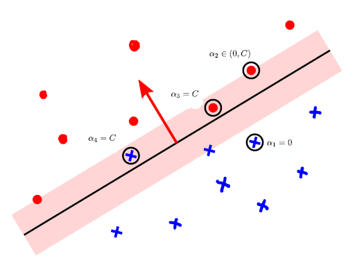
In the figure above, the pink region represents the “margin” created by the SVM. The center of the margin is the separating hyperplane; its direction is perpendicular to $w$ , the normal vector defining the hyperplane. The margin’s total width is $2 / ∥ w ∥$ .

Points inside the margin are feature vectors $x$ for which $∣ ∣ x^{T} w ∣ ∣ < 1$ . These points incur a cost with hinge loss. Any points outside the margin, for which $∣ ∣ x^{T} w ∣ ∣ \geq 1$ , do not incur any cost, as long as they’re on the correct side. Thus, depending on the $w$ that we choose, the orientation and size of the margin will change; there will be a different number of points in it, and the cost will change.

How can we pick a good margin? Let’s assume $λ$ is small; we won’t define that further, the main point is just we pick one with the following priorities (in order):

We want a separating hyperplane
We want a scaling of $w$ so that no point of the data is in the margin
We want the margin to be as wide as possible

With conditions 1 and 2, we can ensure that there is no cost incurred in the first expression (the sum over $[1 - y_{n} x_{n}^{T} w]_{+}$ ). The third condition is ensured by the fact that we’re minimizing ${∥ w ∥}^{2}$ . Since the size of the margin is inversely proportional to that, we’re maximizing the margin.

We’ve introduced SVMs for the general case, where the data is not necessarily linearly separable, which is the soft-margin formulation. In the hard-margin formulation, the data is linearly separable by a separating hyperplane. Maximizing the margin size in the hard-margin formulation implies that some points will lie exactly on the margin boundary (on the correct side). These points are called essential support vectors. For the soft-margin case, this interpretation becomes a little more muddled.

Alternative formulation: Duality

Now that we know what function we’re optimizing, let’s look at how we can optimize it efficiently. The function is convex, and has a subgradient in $w$ , which means we can use SGD with subgradients. This is good news! We’ll discuss an alternative, but equivalent formulation via the concept of duality, which can lead us to a more efficient implementation in some cases. More importantly though, the dual problem can point us to a more general formulation, called the kernel trick.

Let’s say that we’re interested in minimizing a cost function $L (w)$ . Let’s assume this can be defined through an auxiliary function $G$ , such that:

L (w) = max α α G (w, α α)

The minimization in question is thus:

min w L (w) = min w max α α G (w, α α)

We call this the primal problem. In some cases though, it may be easier to find this in the other direction:

max α α min w G (w, α α)

We call this the dual problem. This leads us to a few questions:

How do we find a suitable function G?

There’s a general theory on this topic (see Nonlinear Programming by Dimitri Bertsekas). In the case of SVMs though, the finding the function G is rather straightforward, once we restate the hinge loss as follows:

[z]_{+} = max {0, z} = max α α z, with α \in [0, 1]

The SVM problem then becomes:

\begin{matrix} min w max α α \in [0, 1]^{N} N \sum n = 1 α_{n} (1 - y_{n} x_{n}^{T} w) + \frac{λ}{2} {∥ w ∥}^{2}      G (w, α α) \\ (Primal problem) \end{matrix}

Note that G is convex in $w$ , and linear, hence concave, in $α α$ .

When is it OK to switch min and max?

It is always true that:

max α α min w G (w, α α) \leq min w max α α G (w, α α)

This is proven by:

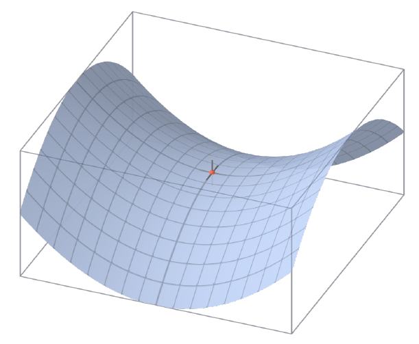
\begin{matrix} min w^{'} G (w^{'}, α α) & \leq G (w, α α) \forall w, α α & ⟺ max α α min w^{'} G (w^{'}, α α) & \leq max α α G (w, α α) \forall w & ⟺ max α α min w^{'} G (w^{'}, α α) & \leq min w max α α G (w, α α) \end{matrix}

Equality is achieved when the function looks like a saddle: when $G$ is a continuous function that is convex in $w$ , concave in $α α$ , and the domains of both are compact and convex.

Saddle function

For SVMs, this condition is fulfilled, and the switch between min and max can be done. The alternative formulation of SVMs is:

\begin{matrix} max α α \in [0, 1]^{N} min w N \sum n = 1 α_{n} (1 - y_{n} x_{n}^{T} w) + \frac{λ}{2} {∥ w ∥}^{2}      G (w, α α) \\ (Dual problem) \end{matrix}

We can take the derivative with respect to $w$ :

\nabla_{w} G (w, α α) = - N \sum n = 1 α_{n} y_{n} x_{n} + λ w

We’ll set this to zero to find a formulation of $w$ in terms of $α$ . We get:

w (α α) = \frac{1}{λ} N \sum n = 1 α_{n} y_{n} x_{n} = \frac{1}{λ} X^{T} Y α α

Where $Y := diag (y)$ . If we plug this into $Dual problem$ , we get the following dual problem, in quadratic form:

\begin{matrix} max α α \in [0, 1]^{N} N \sum n = 1 α_{n} (1 - \frac{1}{λ} y_{n} x_{n}^{T} X^{T} Y α α) + \frac{λ}{2} {∥ ∥ ∥ \frac{1}{λ} X^{T} Y α α ∥ ∥ ∥}^{2} = max α α \in [0, 1]^{N} α α^{T} 1 - \frac{1}{2 λ} α α^{T} {Y X X}^{T} Y α α \\ (Quadratic form) \end{matrix}

When is the dual easier to optimize than the primal?

When the dual is a differentiable quadratic problem (as SVM is). This is a problem that takes the same $Quadratic form$ as above. In this case, we can optimize by using coordinate descent (or more precisely, ascent, as we’re searching for the maximum). Crucially, this method only changes one $α_{n}$ variable at a time.
In the $Quadratic form$ above, the data enters the formula in the form $K = {X X}^{T}$ . This is called the kernel. We say this formulation is kernelized. Using this representation is called the kernel trick, and gives us some nice consequences that we’ll discuss later.
Typically, the solution $α α$ is sparse, being non-zero only in the training examples that are instrumental in determining the decision boundary. If we recall how we defined $α$ in an alternative formulation of $[z]_{+}$ , we can see that there are three distinct cases to consider:
1. Examples that lie on the correct side, and outside the margin, for which $α_{n} = 0$ . These are non-support vectors
2. Examples that are on the correct side and just on the margin, for which $y_{n} x_{n}^{T} w = 1$ , so $α_{n} \in (0, 1)$ . These $x_{n}$ are essential support vectors
3. Examples that are strictly within the margin, or on the wrong side have $α_{n} = 1$ , and are called bound support vectors

Kernel trick

We saw previously that our data only enters $Quadratic form$ in the form of a kernel, $K = {X X}^{T}$ . We’ll see now that when we’re using the kernel, we can easily go to a much larger dimensional space (even infinite dimensional space) without adding any complexity. This isn’t always applicable though, so we’ll also see which kernel functions are admissible for this trick.

Alternative formulation of ridge regression

Let’s recall that least squares is a special case of ridge regression (where $λ = 0$ ). Ridge regression corresponds to the following optimization problem:

w^{*} = min w N \sum n = 1 (y_{n} - x_{n}^{T} w)^{2} + \frac{λ}{2} {∥ w ∥}^{2}

We saw that the solution has a closed form:

w^{*} = (X^{T} X + λ I_{D})^{- 1} X^{T} y

We claim that this can be alternatively written as:

w^{*} = X^{T} ({X X}^{T} X + λ I_{N}      N \times N)^{- 1} y

The original formulation’s runtime is $O (D^{3} + N D^{2})$ , while the alternative is $O (N^{3} + D N^{2})$ . Which is more efficient depends on $D$ and $N$ .

Proof

We can prove this formulation by using the following identity. If we let $P$ be an $N \times M$ matrix, and $Q$ be $M \times N$ . Then:

P (Q P + I_{M}) = P Q P + P = (P Q + I_{N}) P

Assuming that $(Q P + I_{M})$ and $(P Q + I_{N})$ are invertible, we have the identity:

(P Q + I_{N})^{- 1} P = P (Q P + I_{M})^{- 1}

To derive the formula, we can let $P = X^{T}$ and $Q = \frac{1}{λ} X$ .

Representer theorem

The representer theorem generalizes what we just saw about ridge regression. For a $w^{*}$ minimizing the following, for any cost $L_{n}$ ,

min w N \sum n = 1 L_{n} (x_{n}^{T} w, y_{n}) + \frac{λ}{2} {∥ w ∥}^{2}

there exists $α^{*} α^{*}$ such that $w^{*} = X^{T} α α^{*}$ .

Kernelized ridge regression

The above theorem gives us a new way of searching for $w^{*}$ : we can first search for $α^{*} α^{*}$ , which might be easier, and then get back to the optimal weights by using the identity $w^{*} = X^{T} α α^{*}$ .

Therefore, for ridge regression, we can equivalently optimize our alternative formula in terms of $α$ :

α α^{*} = arg min α α \frac{1}{2} α α^{T} ({X X}^{T} + λ I_{N}) α α - α α^{T} y

We see that our data enters in kernel form. How do we get the solution to this minimization problem? We can, as always, take the gradient of the cost function according to $α α$ and set it to zero:

\nabla_{α α} L (α α) = ({X X}^{T} + λ I_{N}) α α - y = 0

Solving for $α$ results in:

\begin{matrix} α α^{*} & = ({X X}^{T} + λ I_{N})^{- 1} y w^{*} & = X^{T} α α^{*} = X^{T} ({X X}^{T} + λ I_{N})^{- 1} y \end{matrix}

We’ve effectively gotten back to our claimed alternative formulation for the optimal weights.

Kernel functions

The kernel is defined as $K = {X X}^{T}$ . We’ll call this the linear kernel. The elements are defined as:

K = {X X}^{T} = ⎡ ⎢ ⎢ ⎢ ⎢ ⎢ ⎢ ⎣ \begin{matrix} x_{1}^{T} x_{1} & x_{1}^{T} x_{2} & \dots & x_{1}^{T} x_{N} x_{2}^{T} x_{1} & x_{2}^{T} x_{2} & \dots & x_{2}^{T} x_{N} ⋮ & ⋮ & ⋱ & ⋮ x_{N}^{T} x_{1} & x_{N}^{T} x_{2} & \dots & x_{N}^{T} x_{N} \end{matrix} ⎤ ⎥ ⎥ ⎥ ⎥ ⎥ ⎥ ⎦

The kernel matrix is a $N \times N$ matrix. Now, assume that we had first augmented the feature space with $ϕ (x)$ ; the elements of the kernel would then be:

K = Φ Φ Φ Φ^{T} = ⎡ ⎢ ⎢ ⎢ ⎢ ⎢ ⎣ \begin{matrix} ϕ (x_{1})^{T} ϕ (x_{1}) & ϕ (x_{1})^{T} ϕ (x_{2}) & \dots & ϕ (x_{1})^{T} ϕ (x_{N}) ϕ (x_{2})^{T} ϕ (x_{1}) & ϕ (x_{2})^{T} ϕ (x_{2}) & \dots & ϕ (x_{2})^{T} ϕ (x_{N}) ⋮ & ⋮ & ⋱ & ⋮ ϕ (x_{N})^{T} ϕ (x_{1}) & ϕ (x_{N})^{T} ϕ (x_{2}) & \dots & ϕ (x_{N})^{T} ϕ (x_{N}) \end{matrix} ⎤ ⎥ ⎥ ⎥ ⎥ ⎥ ⎦

Using this formulation allows us to keep the size of $K$ the same, regardless of how much we augment. In other words, we can now solve a problem where the size is independent of the feature space.

The feature augmentation goes from $x_{n} \in R^{D}$ to $ϕ (x_{n}) \in R^{D^{'}}$ with $D^{'} ≫ D$ , or even to an infinite dimension.

The big advantage of using kernels is that rather than first augmenting the feature space and then computing the kernel by taking the dot product, we can do both steps together, and we can do it more efficiently.

Let’s define a kernel function $κ (x, x^{'})$ . We’ll let entries in the kernel $K$ be defined by:

K_{i, j} = κ (x_{i}, x_{j})

We can pick different kernel functions and get some interesting results. If we pick the right kernel, it can be equivalent to augmenting the features with some $ϕ (x)$ , and then computing the inner product:

κ (x, x^{'}) = ϕ (x)^{T} ϕ (x^{'})

Hopefully, $κ$ is simple enough of a function that it’ll still be easier to compute than going to the higher dimensional space via $ϕ$ and then computing the dot product.

Let’s take a look at a few examples of choices for $κ$ and see what happens. In the following, we’ll go the other way around, picking a $κ$ and showing that it’s equivalent to a particular feature augmentation $ϕ$ .

Trivial kernels

This is the trivial example, in which there is no feature augmentation. The following definition of $κ$ is equivalent to the identity “augmentation”:

κ (x_{1}, x_{2}) = x_{1}^{T} x_{2} ⟹ ϕ (x) = x

Another trivial example assumes that $x_{1}, x_{2} \in R$ . We’ll define the following kernel function, which is equivalent to the feature augmentation that takes the square:

κ (x_{1}, x_{2}) = (x_{1} \cdot x_{2})^{2} ⟹ ϕ (x) = x^{2}

Polynomial kernel

Let’s assume that $x^{'}, x^{'} \in R^{3}$ . Let’s define the kernel function as follows:

\begin{matrix} κ (x, x^{'}) & = {(x_{1} x_{1}^{'} + x_{2} x_{2}^{'} + x_{3} x_{3}^{'})}_{1}^{2} = {(x_{1} x_{1}^{'})}_{1}^{2} + {(x_{2} x_{2}^{'})}_{2}^{2} + {(x_{3} x_{3}^{'})}_{3}^{2} + 2 x_{1} x_{1}^{'} x_{2} x_{2}^{'} + 2 x_{1} x_{1}^{'} x_{3} x_{3}^{'} + 2 x_{2} x_{2}^{'} x_{3} x_{3}^{'} \end{matrix}

What is the $ϕ$ corresponding to this? The inner product that would produce the above would is produced by taking the inner product $ϕ (x)^{T} ϕ (x^{'})$ , where $ϕ$ is defined as follows:

ϕ (x) = [\begin{matrix} \sqrt{2} x_{1} x_{2} & \sqrt{2} x_{1} x_{3} & \sqrt{2} x_{3} x_{3} & x_{1}^{2} & x_{2}^{2} & x_{3}^{2} \end{matrix}]

Radial basis function kernel

The following kernel corresponds to an infinite feature map:

κ (x, x^{'}) = exp [- (x - x^{'})^{T} (x - x^{'})]

This is called the radial basis function (RBF) kernel.

Consider the special case in which $x$ and $x^{'}$ are scalars; we’ll look at the Taylor expansion of the function:

\begin{matrix} κ (x, x^{'}) & = exp [- (x - x^{'})^{2}] = exp [- (x^{2} + (x^{'})^{2} - 2 x x^{'})] = e^{- x^{2}} e^{- (x^{'})^{2}} e^{2 x x^{'}} = e^{- x^{2}} e^{- (x^{'})^{2}} \infty \sum k = 0 \frac{2^{k} (x)^{k} (x^{'})^{k}}{k!} \end{matrix}

We can think of this infinite sum as the dot-product of two infinite vectors, whose $k$ -th components are equal to, respectively:

e^{- x^{2}} \sqrt{\frac{2^{k}}{k!}} x^{k} and e^{- (x^{'})^{2}} \sqrt{\frac{2^{k}}{k!}} (x^{'})^{k}

Although it isn’t obvious, we’ll state that this kernel cannot be represented as an inner product in finite-dimensional space; it is inherently the product of infinite dimensional vectors.

New kernel functions from old ones

We can simply construct a new kernel as a linear combination of old kernels:

\begin{matrix} κ (x, x^{'}) & = a κ_{1} (x, x^{'}) + b κ_{2} (x, x^{'}), & \forall a, b \geq 0 κ (x, x^{'}) & = κ_{1} (x, x^{'}) κ_{2} (x, x^{'}) κ (x, x^{'}) & = κ_{1} (f (x), f (x^{'})), & f : R^{D} \to R^{D} κ (x, x^{'}) & = f (x) f (x^{'}), & in which case ϕ (x) = f (x) \end{matrix}

Proofs are in the lecture notes. If we accept these, we can combine them to prove much more complex kernel functions.

Classifying with the kernel

So far, we’ve seen how to compute the optimal parameter $α α$ using only the kernel, without having to go to the extended feature space. This also allows us to have infinite feature spaces. Now, let’s see how to use all of this to create predictions using only the kernel.

Recall that the classifier predicts $y_{n} = ϕ (x_{n})^{T} w^{*}$ , and that $w^{*} = X^{T} α α^{*}$ . This leads us to:

y_{m} = ϕ (x_{m})^{T} ϕ (X)^{T} α α = N \sum n = 1 κ (x_{m}, x_{n}) α α

Properties of kernels

How can we ensure that there exists a feature augmentation $ϕ$ corresponding to a given kernel $K$ ? A kernel function must be an inner-product in some feature space. Mercer’s condition states that we have this iff the following conditions are fulfilled:

$K$ is symmetric, i.e. $κ (x, x^{'}) = κ (x^{'}, x)$
For any arbitrary input set ${x_{n}}$ and all $N$ , $K$ is positive semi-definite

Unsupervised learning

So far, all we’ve done is supervised learning: we’ve gone from a training set with features vectors and labels, and we wanted to output a classification or a regression.

There is a second very important framework in ML called unsupervised learning. Here, the training set is only composed of the feature vectors; there are no associated labels:

S_{train} = {(x_{n})}_{n}^{N}

We would then like to learn from this dataset without having access to the training labels. The two main directions in unsupervised learning are:

Representation learning & feature learning
Density estimation & generative models

Let’s take a bird’s eye view of the existing techniques through some examples.

Matrix factorization: can be used for both supervised and unsupervised. We’ll give an example for each
1. Netflix, collaborative filtering: this is an example of supervised learning. We have a large, sparse matrix with rows of users, columns of movies, containing ratings. If we can approximate the matrix reasonably well by a matrix of rank one (i.e. outer product of two vectors), then this extracts useful features both for the users and the movies; it might group movies by genres, and users by type.
2. word2vec: this is an example of unsupervised learning. The idea is to map every word from a large corpus to a vector $w_{i} \in R^{K}$ , where K is relatively large. This would allow us to represent natural language in some numeric space. To get this, we build a matrix $N \times N$ , with $N$ being the number of words in the corpus. We then factorize the matrix by means of two matrices of rank $K$ to give us the desired representation. The results are pretty astounding, as this article shows; closely related words are close in the vector space, and it’s easy to get a mapping from concepts to associated concepts (say, countries to capitals).
PCA and SVD (Principle Component Analysis and Singular Value Decomposition): Features are vectors in $R^{d}$ for some d. If we wanted to “compress” this down to one dimension (this doesn’t have to be an existing feature, it could be a newly generated one from the existing ones), we could ask that the variance of the projected data be as large as possible. This will lead us to PCA, which we compute using SVD.
Clustering: to reveal structure in data, we can cluster points given some similarity measure (e.g. Euclidean distance) and the number of clusters we want. We can also ask clusters to be hierarchical (clusters within clusters).
Generative models: a generative model models the distribution of the data
1. Auto-encoders: these are a form of compression algorithm, trying to find good weights for encoding and compressing the data
2. Generative Adversarial Networks (GANs): the idea is to use two neural nets, one that tries to generate samples that look like the data we get, and another that tries to distinguish the real samples from the fake ones. The aim is that after sufficient training, a classifier cannot distinguish real samples from artificial ones. If we achieve that, then we have built a good model.

K-Means

A common algorithm for unsupervised learning is called K-means (also called vector quantization in signal processing, or the Baum-Welch algorithm for hidden Markov models). The aim of this algorithm is to cluster the data: we want to find a partition such that every point is exactly one group, such that within a group, the (Euclidean) distance between points is much smaller than across the groups.

In K-means, we find these clusters in terms of cluster centers $μ μ$ (also called means). Each center dictates the partition: which cluster a point belongs to depends on which center is closest to the point. In other words, we’re minimizing the distance over all $N$ points and $K$ clusters:

min μ μ, z L_{K-means} (z, μ μ) = min {μ μ_{k}}, {z_{n k}} N \sum n = 1 K \sum k = 1 z_{n k} {∥ x_{n} - μ μ_{k} ∥}_{n}^{2}

The $z_{n k}$ is the k^th number in the $z_{n}$ vector, which is a one-hot vector encoding the cluster assignment. Every datapoint $x_{n}$ has an associated vector $z_{n}$ of length K, that takes value 1 in the index of the cluster to which $x_{n}$ belongs, and 0 everywhere else. Mathematically, we can write this constraint as:

z_{n k} \in {0, 1}, K \sum k = 1 z_{n k} = 1

To recap, we have the following vectors:

\begin{matrix} z_{n} & = {[z_{n 1}, z_{n 2}, \dots, z_{n K}]}_{n 1}^{T} z & = {[z_{1}, z_{2}, \dots, z_{N}]}_{1}^{T} μ μ & = {[μ μ_{1}, μ μ_{2}, \dots, μ μ_{K}]}_{1}^{T} \end{matrix}

This formulation of the problem gives rise to two conditions, which will give us an intuitive algorithm for solving this iteratively. We see that there are two sets of variables to optimize under: $μ μ_{k}$ and $z_{n k}$ . The idea is to fix one and optimize the other.

First, let’s fix the centers ${μ μ_{k}}$ and work on the assignments. To minimize the sum:

z_{n k} = {\begin{matrix} 1, & k = {arg min}_{k^{'}} {∥ x_{n} - μ μ_{k^{'}} ∥}_{n}^{2} 0, & otherwise \end{matrix}

Intuitively, this means that we’re grouping the points by the closest center.

Having computed this, we can fix the assignments $z_{n k}$ to compute optimal centers $μ μ_{k}$ . These centers should correspond to the center of the cluster. This minimizes the distance that all points can have to the center.

μ μ_{k} = \frac{\sum_{n = 1}^{N} z_{n k} x_{n}}{\sum_{n = 1}^{N} z_{n k}}

Note that in this formulation, $k$ is fixed by $μ μ_{k}$ , and $n$ varies in the sum. This gives us some kind of average: the sum of all the positions of the points in the cluster, divided by the number of points in the cluster.

How did we get to this formulation? If we take the derivative of the cost function and set it to zero, and then solve it for $μ μ_{k}$ , we get to the above.

\nabla_{μ μ_{k}} L_{K-means} = N \sum n = 1 2 z_{n k} μ μ_{k} - 2 z_{n k} x_{n} = 0

Solving this confirms that taking the average position in the cluster indeed is the best way to optimize our cost.

These observations give rise to an algorithm:

Initialize the centers ${μ μ_{k}^{(0)}}$ . In practice, the algorithm’s convergence may depend on this choice, but there is no general best strategy. As such, they can in general be initialized randomly.
Repeat until convergence:
1. Choose $z^{(t + 1)}$ given $μ μ^{(t)}$
2. Choose $μ μ^{(t + 1)}$ given $z^{(t + 1)}$

Each of these two steps will only make the partitioning better, if possible. Still, this may get stuck at a local minimum, there’s no guarantee of it converging to the global optimum; it’s a greedy algorithm.

Coordinate descent interpretation

There are other ways to look at K-means. One way is to think of it as a coordinate descent, minimizing a cost function by finding parameters $μ μ$ and $z$ iteratively:

\begin{matrix} z^{(t + 1)} & = arg min z L (z, μ μ^{(t)}) μ μ^{(t + 1)} & = arg min μ μ L (z^{(t + 1)}, μ μ) \end{matrix}

This doesn’t actually give us much new insight, but it’s a nice way to think about it.

Matrix factorization interpretation

Another way to think about it is as a matrix factorization. We can rewrite K-means as the following minimization:

min μ μ, z L_{K-means} (z, μ μ) = min M, Z {∥ ∥ X^{T} - M Z^{T} ∥ ∥}_{Frob}^{T}^{2}

A few notes on this notation:

$X$ is, as always, the $N \times D$ data matrix
$M$ is a $D \times K$ matrix representing the mean, the $μ μ_{k}$ vectors; each column represents a different center
$Z^{T}$ is the $K \times N$ assignment matrix containing the $z_{n}$ vectors. This means that the columns of $Z^{T}$ are one-hot vectors, i.e. that exactly one element of each column of $Z^{T}$ is 1
$X^{T} - M Z^{T}$ computes a matrix whose rows are vectors from each point to its corresponding cluster center.
The ${∥ \cdot ∥}_{Frob}$ norm here is the Frobenius norm, the sum of the squares of all elements in matrix. Using the Frobenius norm allows us to get a sum of errors squared, which should be reminiscent of most loss functions we’ve used so far

This is indeed a matrix factorization as we’re trying to find two matrices $M$ and $Z$ that minimize the above criterion.

Probabilistic interpretation

A probabilistic interpretation of K-means will lead us to Gaussian Mixture Models (GMMs). Having a probabilistic approach is useful because it allows us to account for the model that we think generated the data.

The assumption is that we have generated the data by using $K$ separate $D$ -dimensional Gaussian distributions. Each sample $x_{n}$ comes from one of the $K$ distributions uniformly at random. These distributions are assumed to have means ${μ μ_{k}}$ , and the identity matrix as their covariance matrix (that is, variance 1 in each dimension, and the dimensions are i.i.d).

Let’s write down the likelihood of a sample $x_{n}$ . It’s the Gaussian density function of the cluster to which the sample belongs:

p (x_{n} ∣ μ μ, z) = K \prod k = 1 {(\frac{1}{(2 π)^{D / 2}} exp \frac{- {∥ x_{n} - μ μ_{k} ∥}_{n}^{2}}{2})}^{z_{n k}}

The density assuming that we know that the points are from a given $k$ is what’s inside of the large parentheses. We use $z_{n k}$ in the exponent to cancel out the contributions of the clusters to which $x_{n}$ does not belong, keeping only the contribution of its cluster.

Now, if we want the likelihood for the whole set instead of for a single sample, assuming that the samples are i.i.d, we can take the product over all samples:

p (X ∣ μ μ, z) = N \prod n = 1 p (x_{n} ∣ μ μ, z) = N \prod n = 1 K \prod k = 1 {(\frac{1}{(2 π)^{D / 2}} exp \frac{- {∥ x_{n} - μ μ_{k} ∥}_{n}^{2}}{2})}^{z_{n k}}

This is the likelihood, which we want to maximize. We could equivalently minimize the log-likelihood. We’ll also remove the constant factor as it has no influence on our minimization.

\begin{matrix} - log p (X ∣ μ μ, z) & = - log N \prod n = 1 p (x_{n} ∣ μ μ, z) = - log N \prod n = 1 K \prod k = 1 {(exp \frac{- {∥ x_{n} - μ μ_{k} ∥}_{n}^{2}}{2})}^{z_{n k}} = N \sum n = 1 K \sum k = 1 z_{n k} {∥ x_{n} - μ μ_{k} ∥}_{n}^{2} \end{matrix}

And this is of course the cost function we were optimizing before.

Issues with K-means

Computation may be heavy for large values of $N$ , $D$ and $K$
Clusters are forced to be spherical (and cannot be elliptical for instance)
Each input can belong to only one cluster (this is known as “hard” cluster assignment, as opposed to “soft” assignment which allows for weighted memberships in different clusters)

Gaussian Mixture Model (GMM)

So now that we’ve expressed K-means from a probabilistic view, let’s view the probabilistic generalization, which is called a Gaussian Mixture Model.

Clustering with Gaussians

To generalize the previous, what if our data comes from Gaussian sources that aren’t perfectly circularly symmetric¹⁰, that don’t have the identity matrix as variance? A more general solution is to allow for an arbitrary covariance matrix $Σ Σ_{k}$ . This will add another parameter that we need optimize over, but can help us more accurately model the data.

Soft clustering

Another extension is that we were previously forced to be either from one or another distribution. This is called hard clustering. We can generalize this to soft clustering, where a point can be associated to multiple clusters. In soft clustering, we model $z_{n}$ as a random variable taking values in ${1, \dots, K}$ , instead of a one-hot vector $z_{n}$ .

This assignment is given by a certain distribution. We denote the prior probability that the sample comes from the k^th Gaussian $N (μ μ_{k}, Σ Σ_{k})$ , by $π_{k}$ :

p (z_{n} = k) = π_{k}, where π_{k} > 0 \forall k and K \sum k = 1 π_{k} = 1

Likelihood

What we’re trying to minimize in this extended model is then (still under the assumption that the data is independently distributed from $K$ samples):

\begin{matrix} p (X, z ∣ μ μ, Σ Σ, π π) & = N \prod n = 1 p (z_{n} ∣ π π) N (x_{n} ∣ z_{n}, μ μ, Σ Σ) = N \prod n = 1 K \prod k = 1 {(π_{k} N (x_{n} ∣ μ μ_{k}, Σ Σ_{k}))}_{k}^{z_{n k}} \end{matrix}

Our notation here maybe isn’t the best; we’re still using $z_{n k}$ as an indicator, but also $z_{n}$ as a random variable, and not a one-hot vector anymore. Therefore, to be clear, we should define $z_{n k} = I {z_{n} = k}$ .

This is the model that we’ll use. It’s not something that we aim to prove or not prove, it’s just what we chose to base ourselves on. We’ll want to optimize over $μ μ$ and $Σ Σ$ .

The $z_{n}$ variable is what’s known asf a latent variable; it’s not something that we observe directly, it’s just something that we use to make our model more complex. The parameters of the model are $θ θ := {μ μ, Σ Σ, π π}$ .

Marginal likelihood

The advantage of treating $z_{n}$ are latent variables instead of parameters is that we can marginalize them out to get a cost function that doesn’t depend on them. If we’re not interested in these latent variables, we can integrate over the latent variables to get the marginal likelihood:

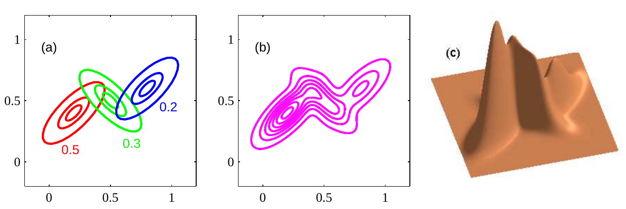
p (X ∣ θ θ) = N \prod n = 1 p (x_{n} ∣ θ θ) = N \prod n = 1 K \sum k = 1 π_{k} N (x_{n} ∣ μ μ_{k}, Σ Σ_{k})

2D view of weighted gaussians forming a single distribution — Multiple Gaussians form a single distribution in GMM

This is a weighted sum of all the models. The weights sum up to one, so we have a valid density. In other words, we are now able to model much more complex distribution functions by building up our distribution from $K$ Gaussian distributions.

Weighted Gaussian bell curves — The $π_{k}$ factors allow us to weigh multiple Gaussian distributions

Assuming that $D, K ≪ N$ , the number of parameters in the model was $O (N)$ , because we had an assignment $z_{n}$ for each of the $N$ datapoints. Now, assignments are no longer a parameter, so the number of parameters grows in $O (D^{2} K)$ , since we have $K$ covariance matrices, which are $D \times D$ , and $K$ $D$ -dimensional clusters. Under our assumption that $D, K ≪ N$ , having $O (D^{2} K)$ parameters is much better.

Maximum likelihood

We can optimize the fit of the model by changing the parameters of $θ θ$ and optimizing the log likelihood of the above, which is:

^θ θ = max θ θ N \sum n = 1 log (K \sum k = 1 π_{k} N (x_{n} ∣ μ μ_{k}, Σ Σ_{k}))

This can be optimized over $π_{k}, μ μ_{k}, Σ Σ_{k}$ . Unfortunately, we now have the log of a sum of Gaussians (which are exponentials), which isn’t a very nice formula. We’ll use this as an excuse to talk about another algorithm, the EM algorithm.

EM algorithm

In GMM, we had the following set of parameters:

θ θ^{(t)} := {{μ μ_{k}^{(t)}}_{k = 1}^{K}, {Σ Σ_{k}^{(t)}}_{k = 1}^{K}, {π_{k}^{(t)}}_{k = 1}^{K}}

We wanted to optimize these parameters under the following maximization problem:

max θ θ L (θ θ) = max θ θ N \sum n = 1 log (K \sum k = 1 π_{k} N (x_{n} ∣ μ μ_{k}, Σ Σ_{k}))

Note that in this problem, we’re maximizing the cost function instead of minimizing it as we’re used to. This is strictly equivalent to minimizing the negative of this, and we’re using maximizing and minimizing the negative equivalently.

This is not an easy optimization problem, because wee need to optimize the logarithm of a sum over all choices of $θ θ$ .

The expectation-maximization (EM) algorithm provides with a general method to tackle this kind of problem. It uses an iterative two-step algorithm: at every step, we try to go from a set of parameters $θ θ^{(t)}$ to a better set of parameters $θ θ^{(t + 1)}$ .

In the following, we’ll consider an arbitrary probability distribution $q_{n}^{(t)}$ over $K$ members. Since it is a probability distribution, we have:

q_{n k}^{(t)} \geq 0, K \sum k = 1 q_{n k}^{(t)} = 1

The EM algorithm consists of optimizing for $q_{n k}$ and $θ θ$ alternatively. Note that while every step improves the cost, there is no guarantee that this will converge to the global optimum.

We start by initializing $μ μ^{(0)}, Σ Σ^{(0)}, π π^{(0)}$ . Then, we iterate between the E and M steps until $L (θ θ)$ stabilizes.

Expectation step

In the expectation step, we compute how well we’re doing:

L (θ θ^{(t)}) = N \sum n = 1 log (K \sum k = 1 π_{k}^{(t)} N (x_{n} ∣ μ μ_{k}^{(t)}, Σ Σ_{k}^{(t)}))

We can then choose the new $q_{n k}^{(t)}$ values:

q_{n k}^{(t)} = \frac{π_{k}^{(t)} N (x_{n} ∣ μ μ_{k}^{(t)}, Σ Σ_{k}^{(t)})}{\sum_{k = 1}^{K} π_{k}^{(t)} N (x_{n} ∣ μ μ_{k}^{(t)}, Σ Σ_{k}^{(t)})}

This gives us a new lower bound on the cost:

L (θ θ^{(t + 1)}) \geq N \sum n = 1 K \sum k = 1 q_{n k}^{(t + 1)} log ⎛ ⎝ \frac{π_{k} N (x_{n} ∣ μ μ_{k}, Σ Σ_{k})}{q_{n k}^{(t + 1)}} ⎞ ⎠

Getting a lower bound means that we have a monotonically non-decreasing cost over the steps $t$ . Again, this is a good guarantee because we’re maximizing over the cost: it tells us that our E-step improves at every step.

This value is actually the expected value, hence the name of the E-step. We’ll see this in the interpretation section below.

Derivation

Due to the concavity of the log function, we can apply Jensen’s inequality recursively to the cost function to get:

\begin{matrix} log (K \sum k = 1 π_{k} N (x_{n} ∣ μ μ_{k}, Σ Σ_{k})) & = log ⎛ ⎝ K \sum k = 1 q_{n k}^{(t)} \frac{π_{k} N (x_{n} ∣ μ μ_{k}, Σ Σ_{k})}{q_{n k}^{(t)}} ⎞ ⎠ \geq K \sum k = 1 q_{n k}^{(t)} log \frac{π_{k} N (x_{n} ∣ μ μ_{k}, Σ Σ_{k})}{q_{n k}^{(t)}} \end{matrix}

Just like in the log-sum inequality, we have equality when the terms in the log are equal for all members of the sum. If that is the case, it means that all these terms are the same scalar, and therefore that the numerator and denominator are proportional:

q_{n k}^{(t)} \propto π_{k} N (x_{n} ∣ μ μ_{k}, Σ Σ_{k})

Since $q_{n k}$ is a probability, it must sum up to 1 so we have:

q_{n k}^{(t)} = \frac{π_{k} N (x_{n} ∣ μ μ_{k}, Σ Σ_{k})}{\sum_{k = 1}^{K} π_{k} N (x_{n} ∣ μ μ_{k}, Σ Σ_{k})}

Maximization step

We update the parameters $θ θ$ as follows:

\begin{matrix} μ μ_{k}^{(t + 1)} & := \frac{\sum_{n} q_{n k}^{(t)} x_{n}}{\sum_{n} q_{n k}^{(t)}} Σ Σ_{k}^{(t + 1)} & := \frac{\sum_{n} q_{n k}^{(t)} (x_{n} - μ μ_{k}^{(t + 1)}) (x_{n} - μ μ_{k}^{(t + 1)})^{T}}{\sum_{n} q_{n k}^{(t)}} π_{k}^{(t + 1)} & := \frac{1}{N} \sum n q_{n k}^{(t)} \end{matrix}

Derivation

We had previously let $q_{n k}$ be an abstract, undefined distribution. We now freeze the $q_{n}^{(t)}$ assignments, and optimize over $θ θ$ .

In the E step, we derived a lower bound for the cost function. In general, the lower bound is not equal to the original cost. We can however carefully choose $q_{n k}$ to achieve equality. And since we want to maximize the original cost function, it makes sense to maximize this lower bound. Thus, we’ll work under this locked assignment of $q_{n k}$ (thus achieving equality for the lower bound). Seeing that we have equality, our objective function (which we want to maximize) is:

N \prod n = 1 K \sum k = 1 q_{n k}^{(t)} log \frac{π_{k} N (x_{n} ∣ μ μ_{k}, Σ Σ_{k})}{q_{n k}^{(t)}}

This leads us to maximizing the expression:

N \sum n = 1 K \sum k = 1 q_{n k}^{(t)} [log π_{k} - log q_{n k}^{(t)} + log N (x_{n} ∣ μ μ_{k}, Σ Σ_{k})]

The $π_{k}$ should sum up to one, so we’re dealing with a constrained optimization problem. We therefore add a term to turn it into an unconstrained problem. We therefore want to maximize the following over $θ θ$ :

N \sum n = 1 K \sum k = 1 q_{n k}^{(t)} [log π_{k} - log q_{n k}^{(t)} + log N (x_{n} ∣ μ μ_{k}, Σ Σ_{k})] + λ K \sum k = 1 π_{k}

Differentiating with respect to $π_{k}$ , and setting the result to 0 yields:

N \sum n = 1 q_{n k}^{(t)} \frac{1}{π_{k}} + λ = 0

Solving for $π_{k}$ gives us:

π_{k} = - \frac{1}{λ} N \sum n = 1 q_{n k}^{(t)}

We can choose $λ$ so that this leads to a proper normalization ( $π_{k}$ summing up to 1); this leads us to $λ = - N$ . Hence, we have:

π_{k}^{(t + 1)} := \frac{1}{N} N \sum n = 1 q_{n k}^{(t)}

This is our first update rule. Let’s see how to derive the others. The term $log N (x_{n} ∣ μ μ_{k}, Σ Σ_{k})$ has the form:

- \frac{D}{2} log (2 π) + \frac{1}{2} log ∣ ∣ Σ Σ^{- 1} ∣ ∣ - \frac{1}{2} (x - μ μ_{k})^{T} Σ Σ^{- 1} (x - μ μ_{k})

We used the fact that for an invertible matrix, $| Σ Σ | = 1 / ∣ ∣ Σ Σ^{- 1} ∣ ∣$ . Differentiating the cost function with respect to $μ μ_{k}$ and setting the result to 0 yields:

N \sum n = 1 q_{n k}^{(t)} Σ Σ^{- 1} (x_{n} - μ μ_{k}) = 0

We can multiply this by $Σ Σ$ on the left to get rid of the $Σ Σ^{- 1}$ , and solve for $μ μ_{k}$ to get:

μ μ_{k}^{(t + 1)} := \frac{\sum_{n} q_{n k}^{(t)} x_{n}}{\sum_{n} q_{n k}^{(t)}}

Finally, for the $Σ Σ$ update rule, we take the derivative with respect to $Σ Σ_{k}^{- 1}$ and set the result to 0, yielding:

N \sum n = 1 q_{n k}^{(t)} \frac{1}{2} Σ Σ_{k}^{T} - \frac{1}{2} N \sum n = 1 q_{n k}^{(t)} (x_{n} - μ μ_{k}) (x_{n} - μ μ_{k})^{T} = 0

Solving for $Σ Σ$ yields:

Σ Σ_{k}^{(t + 1)} := \frac{\sum_{n} q_{n k}^{(t)} (x_{n} - μ μ_{k}^{(t + 1)}) (x_{n} - μ μ_{k}^{(t + 1)})^{T}}{\sum_{n} q_{n k}^{(t)}}

We’re using the following fact, which I won’t go into details to prove:

\frac{\partial}{\partial A} log | A | = A^{- T}

Interpretation

The original model for GMM was that our data points are i.i.d. from a mixture model with $K$ Gaussian components. This led us to the following choice of prior distribution:

\begin{matrix} p (x_{n} ∣ θ θ) & = K \sum k = 1 p (x_{n}, z_{n} = k ∣ θ θ) = K \sum k = 1 p (z_{n} = k ∣ θ θ) p (x_{n} ∣ z_{n} = k, θ θ) = K \sum k = 1 π_{k} N (x_{n} ∣ μ μ_{k}, Σ Σ_{k}) \end{matrix}

Note that we can generalize the EM algorithm to other choices of $p (x_{n}, z_{n} = k ∣ θ θ)$ , but that this is the one we used here.

This probability is an expectation based on the prior $π_{k}$ . Let’s now look at the posterior distribution of $z_{n}$ , given the datapoints $x_{n}$ :

\begin{matrix} p (z_{n} = k ∣ x_{n}, θ θ) & = \frac{p (z_{n} = k, x_{n}, θ θ)}{p (x_{n}, θ θ)} = \frac{p (z_{n} = k, x_{n} ∣ θ θ)}{p (x_{n} ∣ θ θ)} = \frac{p (z_{n} = k, ∣ θ θ) p (x_{n} ∣ z_{n} = k, θ θ)}{p (x_{n} ∣ θ θ)} = \frac{p (z_{n} = k, ∣ θ θ) p (x_{n} ∣ z_{n} = k, θ θ)}{\sum_{j = 1}^{K} p (z_{n} = j ∣ θ θ) p (x_{n} ∣ z_{n} = j, θ θ)} = \frac{π_{k} N (x ∣ μ_{k}, Σ Σ_{k})}{\sum_{j = 1}^{K} π_{j} N (x ∣ μ_{j}, Σ Σ_{j})} =: q_{n k} \end{matrix}

The distribution that we previously just explained as an abstract, unknown distribution is in fact the posterior $p (z_{n} = k ∣ x_{n}, θ θ)$ .

We can now explain why the E step is the expectation step. Assume that we know the $q_{n k}$ (as a thought experiment, imagine a genie told us the assignment probabilities of each sample $x_{n}$ to a component $k$ , which is exactly what the $q_{n k}$ quantities are).

As a reminder, the log-likelihood is:

\begin{matrix} log p (x_{n}, z_{n} = k ∣ θ θ) & = log (p (z_{n} = k ∣ θ θ) p (x_{n} ∣ μ μ_{k}, Σ Σ_{k})) = log (π_{k} N (x_{n} ∣ μ μ_{k}, Σ Σ_{k})) \end{matrix}

Given the parameters $θ θ$ , the expected value of the above log-likelihood, over the distribution of $z_{n}$ , is:

E_{z_{n}} [log p (x_{n}, z_{n} = k ∣ θ θ)] = K \sum k = 1 q_{n k} log π_{k} N (x_{n} ∣ μ μ_{k}, Σ Σ_{k})

Summing this over all samples $x_{n}$ , we find the cost

N \sum n = 1 K \sum k = 1 q_{n k} log π_{k} N (x_{n} ∣ μ μ_{k}, Σ Σ_{k})

This is almost the same as the expression we maximized in the derivation for the M step, modulo the terms $- q_{n k} log (q_{n k})$ , which are just constants for the maximization.

With this probabilistic interpretation, can write the whole EM algorithm compactly as:

θ θ^{(t + 1)} = arg max θ θ E_{p (z_{n} ∣ x_{n}, θ θ^{(t)})} [log p (x_{n}, z_{n} ∣ θ θ)]

Matrix Factorization

Matrix factorization is a form of unsupervised learning. A well-known example in which matrix factorization was used is the Netflix prize. The goal was to predict ratings of users for movies, given a very sparse matrix of ratings. We’ll study the method that achieved the best error.

Let’s describe the data a little more formally. Given movies $d = 1, 2, \dots, D$ and users $n = 1, 2, \dots, N$ , we define $X$ as the $D \times N$ matrix¹¹ containing all rating entries; that is, $x_{d n}$ is the rating of the n^th user for the d^th movie. We don’t have any additional information on the users or on the movies, apart from the ID that’s been assigned to them. In practice, the matrix was $D = 20^{'} 000$ and $N = 500^{'} 000$ , and 99.98% unobserved.

We want to give a prediction for all the unobserved entries, so that we can give the top entries (say, top 10 movies) for each user.

Prediction using a matrix factorization

We will aim to find $W$ and $Z$ such that:

X \approx W Z^{T}

The hope is to “explain” each rating $x_{d n}$ by a numerical representation of the corresponding movie and user.

Here, we have a “tall” matrix $W \in R^{D \times K}$ , and $Z \in R^{N \times K}$ , forming a “flat matrix” $Z^{T} \in R^{K \times N}$ . In practice, compared to the size of $N$ or $D$ , $K$ will be relatively small (maybe 50 or so).

We’ll assign a cost function that we’re trying to optimize:

min W, Z L (W, Z) := min W, Z \frac{1}{2} \sum (d, n) \in Ω {[x_{d n} - ({W Z}^{T})_{d n}]}_{d n}^{2}

Here, $Ω \subseteq [D] \times [N]$ is given. It collects the indices of the observed ratings of the input matrix $X$ . Our cost function here compares the number of stars $x_{d n}$ a user assigned to a movie, to the prediction of our model ${W Z}^{T}$ , by using mean squares.

To optimize this cost function, we need to know whether it is jointly convex with respect to $W$ and $Z$ , and whether it is identifiable (there is a unique minimum).

We won’t go into the full proof, but the answer is the minimum is not unique. Since ${W Z}^{T}$ is a product, we could just divide one by 10 and multiply the other by 10 to get a different solution with the same cost.

And in fact, it’s not even convex. We could compute the Hessian, which is:

[\begin{matrix} 0 & 1 1 & 0 \end{matrix}]

This isn’t positive semi-definite, and therefore the product isn’t convex.

If we think of $W$ and $Z$ as numbers (or as $1 \times 1$ matrices), we can give a simpler explanation, that also gives us the intuition for why this isn’t convex. The function $w \cdot z$ looks like a saddle function, and therefore isn’t convex.

Choosing K

$K$ is the number of latent features. This is comparable to the K we chose in K-means, defining the number of clusters. Large values of K facilitate overfitting.

Regularization

We can add a regularizer and minimize the following cost:

L (W, Z) = \frac{1}{2} \sum (d, n) \in Ω {[x_{d n} - ({W Z}^{T})_{d n}]}_{d n}^{2} + \frac{λ_{w}}{2} {∥ W ∥}_{Frob}^{2} + \frac{λ_{z}}{2} {∥ Z ∥}_{Frob}^{2}

With scalars $λ_{w}, λ_{z} > 0$ .

Stochastic gradient descent

With our cost functions in place, we can look at our standard algorithm for minimization. We’ll define loss as a sum of many individual loss functions:

L (W, Z) = \sum (d, n) \in Ω f_{d, n} (W, Z) = \sum (d, n) \in Ω \frac{1}{2} {[x_{d n} - ({W Z}^{T})_{d n}]}_{d n}^{2}

Let’s derive the stochastic gradient for an individual loss function (which is what we need to compute when doing SGD). Matrix calculus is not easy, but understanding it starts with understanding the following sentence: a gradient with respect to a matrix is a matrix of gradients. If we compute the gradient of a function $f$ with respect to a matrix $X \in R^{D \times N}$ , we get a gradient matrix $g \in R^{D \times N}$ , where each element $g_{a, b}$ is the derivative of $f$ with respect to the $(a, b)$ element of $X$ :

g_{a, b} = \frac{\partial f}{\partial x_{a, b}}

Before we find the stochastic gradient, let’s start by just looking at the dimensions of what we’re going to compute:

\begin{matrix} \nabla_{W} f_{d, n} & \in R^{D \times K} \nabla_{Z} f_{d, n} & \in R^{N \times K} \end{matrix}

Luckily, we’re not doing the full gradient here, but only the stochastic gradient, which only requires computing a single entry in the gradient matrix. Therefore, for a fixed pair $(d, n)$ (that is, a rating from user $n$ of movie $d$ ), we will compute a single entry $(d^{'}, k)$ in the $W$ derivative:

{(\nabla_{W} f_{d, n})}_{(d^{'}, k)} = \frac{\partial f_{d, n}}{\partial w_{d^{'}, k}} (W, Z) = {\begin{matrix} - [x_{d n} - ({W Z}^{T})_{d n}] z_{n, k} & if d^{'} = d 0 & otherwise \end{matrix}

The same goes for the derivative by $Z$ . We’ll compute a single entry $(n^{'}, k)$ in $\nabla_{W} f_{d, n}$ :

{(\nabla_{Z} f_{d, n})}_{(n^{'}, k)} = \frac{\partial f_{d, n}}{\partial z_{n^{'}, k}} (W, Z) = {\begin{matrix} - [x_{d n} - ({W Z}^{T})_{d n}] w_{d, k} & if n^{'} = n 0 & otherwise \end{matrix}

With these, we have the formulation for the whole matrices.

It turns out that computing this is very cheap: $O (K)$ . This is the greatest advantage of using SGD for this. There are no guarantees that this works though; this is still an open research question. But in practice, it works really well.

The update step is then:

W^{(t + 1)} = W^{(t)} - γ \nabla_{W} f_{d, n} Z^{(t + 1)} = Z^{(t)} - γ \nabla_{Z} f_{d, n}

With stochastic gradient descent, we only compute the gradient of a single $f_{d, n}$ instead of the whole cost $L$ . Therefore, each step only updates the d^th row of $W$ , and the n^th row of $Z$ .

Alternating least squares (ALS)

The alternating minimization algorithm alternates between optimizing $Z$ and $W$ . ALS is a special case of this, with square error.

No missing entries

For simplicity, let’s just assume that there are no missing entries in the data matrix, that is $Ω = [D] \times [N]$ (instead of $\subseteq$ ). This makes our life a little easier, and we’ll be able to find a closed form solution (indeed, if $Ω$ is the whole set, the problem is pretty easy to solve; if it’s an arbitrary subset, it becomes a NP-hard problem). Our cost is then:

\begin{matrix} L (W, Z) & = \frac{1}{2} D \sum d = 1 N \sum n = 1 {[x_{d n} - ({W Z}^{T})_{d n}]}_{d n}^{2} + \frac{λ_{w}}{2} {∥ W ∥}_{Frob}^{2} + \frac{λ_{z}}{2} {∥ Z ∥}_{Frob}^{2} = \frac{1}{2} {∥ ∥ X - {W Z}^{T} ∥ ∥}_{Frob}^{T} + \frac{λ_{w}}{2} {∥ W ∥}_{Frob}^{2} + \frac{λ_{z}}{2} {∥ Z ∥}_{Frob}^{2} \end{matrix}

ALS then does a coordinate descent to minimize the cost (plus a regularizer). First, we fix $W$ and compute the minimum with respect to $Z$ (we ignore the other regularizer, as minimization is the same with or without an added constant):

min Z \frac{1}{2} {∥ ∥ X - {W Z}^{T} ∥ ∥}_{Frob}^{T} + \frac{λ_{z}}{2} {∥ Z ∥}_{Frob}^{2}

Then, we alternate, minimizing $W$ and fixing $Z$ :

min W \frac{1}{2} {∥ ∥ X - {W Z}^{T} ∥ ∥}_{Frob}^{T} + \frac{λ_{w}}{2} {∥ W ∥}_{Frob}^{2}

These are two least squares problems. The only difference is that we’re searching for a whole matrix in this case, unlike in least squares where we searched for a vector. Still, we can find a closed form for it by setting the gradient with respect to $W$ and then $Z$ to 0, which will give:

\begin{matrix} (Z^{*})^{T} & := (W^{T} W + λ_{z} I_{K})^{- 1} W^{T} X (W^{*})^{T} & := (Z^{T} Z + λ_{w} I_{K})^{- 1} Z^{T} X^{T} \end{matrix}

Note that the regularization helps us make sure that problem indeed is invertible (since we’re adding an identity matrix). This means that we can find a closed form solution if we don’t have any missing entries.

The cost of finding the solution in each step is then per column, $O (N)$ and $O (D)$ , which is not quite as good as the $O (K)$ with SGD. Additionally, we need to construct $W^{T} W$ and $Z^{T} Z$ , which is $O (D^{2})$ . The inversion isn’t too bad: we’re only inverting a $K \times K$ matrix, which is much nicer than dealing with $D$ or $N$ . Also note that there is no step size to tune, which makes it easier to deal with (though slower!).

Missing entries

As before, we can derive the ALS updates for the more general setting, where we only have certain ratings $(d, n) \in Ω$ . The idea is to compute the gradient with respect to each group of variables, and set it to zero.

Text representation learning

Co-occurrence matrix

To attempt to get the meaning of words, we can start by constructing co-occurrence counts from a big corpus or text. This is a matrix $N$ in which $n_{i j}$ is the number of contexts where word $w_{i}$ occurs together with word $w_{j}$ . A context is a window of words occurring together (it could be a document, paragraph, sentence, or a window of $n$ words).

For a vocabulary $ν = {w_{1}, \dots, w_{D}}$ and context words $w_{n} = 1, 2, \dots N$ , the co-occurrence matrix is a very sparse $D \times N$ .

Motivation

We can’t plug string-encoded words directly into our learning models. Can we find a meaningful numerical representation for all of our data? We’d like to find a mapping, or embedding, for each word $w_{i}$ :

w_{i} \mapsto w_{i} \in R^{K}

To construct a word embedding, we want to find a factorization of the co-occurrence matrix $N$ . Typically, we actually use $X = log N$ as the element-wise log of the co-occurrence matrix, i.e. $x_{d n} := log (n_{d n})$ . We’ll find a factorization such that:

X \approx W Z^{T}

As before, we let $Ω \subseteq [D] \times [N]$ collect the indices of non-zero counts in $X$ . In other words, $Ω$ contains indices of word pairs that have been observed in the same context.

For each pair of observed words $(w_{d}, w_{n}) \in Ω$ , we’ll try to explain their co-occurrence count by a numerical representation of the two words; the d^th row of $W$ is the representation of a word $w_{d}$ , and n^th row of $Z$ is the representation of a context word $w_{n}$ .

Bag of words

The naive approach would be to pick $K$ to be the size of the vocabulary, $K = | ν |$ . We can then encode words $w_{i}$ as one-hot vectors taking value 1 at index $i$ . This works nicely, but has high dimensionality, and cannot capture the order of the words, which is why it’s called the bag of words approach.

But we can do this in smarter way. The idea is to pick a much lower $K$ , and try to group semantically similar words in this $K$ -dimensional space.

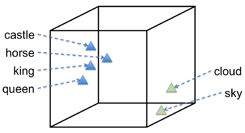
Words with different semantic meanings in different areas of hyperspace

Word2vec

word2vec is an implementation of the skip-gram model. This model uses binary classification (like logistic regression) to separate real word pairs $(w_{d}, w_{n})$ appearing together in a context window, from fake word pairs $(w_{d}, w_{n^{'}})$ .

It does so by computing the inner product score of the words; $w_{d}^{T} w_{n}$ is real, and must be distinguished from the fake $w_{d}^{T} w_{n^{'}}$ .

GloVe

In the following, we’ll give an overview of the method known as GloVe (Global Vectors), which offers an alternative to word2vec.

To do this, we do the following cost minimization:

min W, Z L (W, Z) := min W, Z \frac{1}{2} \sum (d, n) \in Ω f_{d n} {(x_{d n} - (W Z^{T})_{d n})}_{d n}^{2}

The GloVe embedding uses a little trick to weight the importance of each entry. It computes a weight $f_{d n}$ used in the cost above, according to the following function:

f_{d n} = min {1, {(\frac{n_{d n}}{n_{max}})}^{α}}, α \in [0, 1], e.g. α = \frac{3}{4}

Where $n_{max}$ is a parameter to be tuned, and $n_{d n}$ is the count of $w_{d}$ and $w_{n}$ appearing together (not the log, just the normal count). This is a carefully chosen function by the GloVe creators; we can also choose $f_{d n} := 1$ if we don’t want to weigh the vectors, but GloVe achieves good results with this choice.

Glove weight function

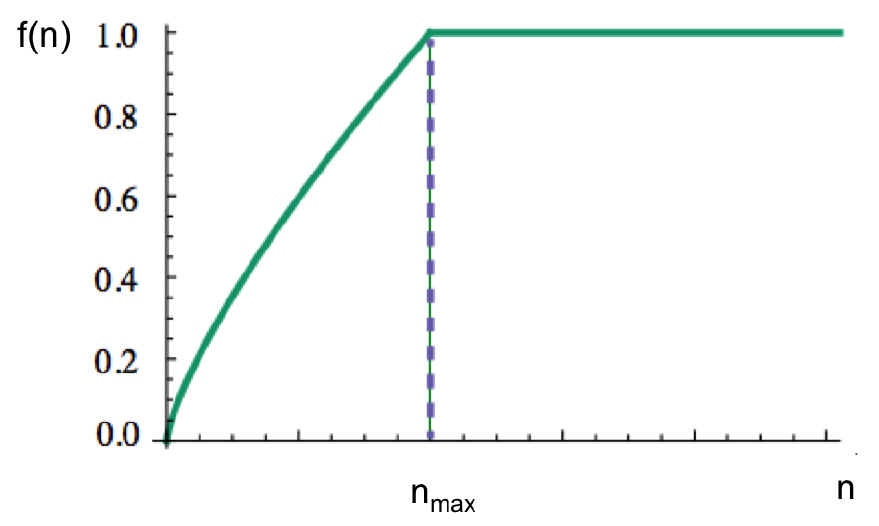
For $K$ , we can just choose a value, say 50, 100 or 200. Trial and error will serve us well here.

We can train the factorization with SGD or ALS.

FastText

This is another matrix factorization approach to learn document or sentence representations. Unlike the two previous approaches, FastText is a supervised algorithm.

A sentence $s_{n}$ is composed of $m$ words: $s_{n} = {w_{1}, w_{2}, \dots, w_{m}}$ . We try to optimize over the following cost function:

min W, Z L (W, Z) := min W, Z \sum s_{n} a sentence f (y_{n} {W Z}^{T} x_{n})

Where:

$W \in R^{1 \times K}$ and $Z \in R^{| ν | \times K}$ are the factorization
$x_{n} \in R^{| ν |}$ is the bag-of-words representation of sentence $s_{n}$
$f$ is a linear classifier loss function, such as the logistic function or hinge loss
$y_{n} \in {\pm 1}$ is the classification label for sentence $s_{n}$

SVD and PCA

Motivation

Principal Component Analysis (PCA) is a popular dimensionality reduction method. Given a data matrix, we’re looking for a way to linearly map the original $D$ dimensions into $K$ dimensions, with $K \leq D$ . The criteria for a good such mapping is that the $K$ -dimensional representation should represent the original data well.

There are different ways to think of PCA:

It compresses data from $K$ to $D$ dimensions
It decorrelates data, finding a $K$ -dimensional space with maximum variance

For machine learning, it’s often best not to compress data in this manner, but it may be necessary in certain situations (for reasons of interpretability for example).

In our subsequent discussion, $X$ is the $D \times N$ data matrix, whose $N$ columns represent the feature vectors in $D$ -dimensional space.

The PCA will be computed from the data matrix $X$ using singular value decomposition.

SVD

The singular value decomposition (SVD) of a $D \times N$ matrix $X$ is:

X = {U S V}^{T}

The matrices

$U$ is a $D \times D$ orthonormal¹² matrix
$V$ is a $N \times N$ orthonormal matrix
$S$ is a $D \times N$ diagonal matrix (with $D$ diagonal entries)

One useful property about unitary matrices (like $U$ and $V$ , which are orthonormal, a stronger claim) is that they preserve the norms (they don’t change the length of the vectors being transformed), meaning that we can think of them as a rotation. A small proof of this follows:

{∥ U x ∥}_{Frob}^{2} = x^{T} U^{T} U x = x^{T} I x = {∥ x ∥}_{Frob}^{2}

We’ll assume $D < N$ without loss of generality (we could just take the transpose of $X$ otherwise). This is an arbitrary choice, but helps us tell the dimensions apart.

The diagonal entries in $S$ are the singular values in descending order:

s_{1} \geq s_{2} \geq \dots \geq s_{D} \geq 0

The columns of $U$ and $V$ are the left and right singular vectors.

SVD and dimensionality reduction

Suppose we want to compress a $D \times N$ data matrix $X$ to a $K \times N$ matrix $~ X$ , where $1 \leq K \leq D$ . We’ll define this transformation from $X$ to $~ X$ by the $K \times D$ compression matrix $C$ . The decompression (or reconstruction) from $~ X$ to $X$ is $R$ .

Can we find good matrices? Our criteria is that the error introduced when compressing and reconstructing should be small, over all choices of compression and reconstruction matrices:

{∥ X - R C X ∥}_{Frob}^{2}

There are other ways of measuring the quality of a compression and reconstruction, but for the sake of simplicity, we’ll stick to this one.

We can actually place a bound on the reconstruction error using the following lemma.

Lemma: For any $D \times N$ matrix $X$ and any $D \times N$ rank-K matrix $^X$ :

{∥ ∥ X -^X ∥ ∥}_{Frob}^{2} \geq {∥ ∥ X - U_{K} U_{K}^{T} X ∥ ∥}_{Frob} = \sum i \geq K + 1 s_{i}^{2}

Where:

$X = U S V^{T}$ is the SVD of $X$
$s_{i}$ are the singular values of $X$
$U_{K}$ is the $D \times K$ matrix of the first $K$ rows of $U$

If we use $C = U_{K}^{T}$ as our compression matrix, and $R = U_{K}$ as the reconstruction matrix, we get a better (or equal) error than any other choice of reconstruction $^X$ . This tells us that the best compression to dimension $K$ is a projection onto the first $K$ columns of $U$ , which are the first $K$ left singular vectors.

Note that the reconstruction error is the sum of the singular values after the cut-off $K$ ; intuitively, we can think of the error as coming from the singular values we ignored.

This also tells us that the left singular vectors are ordered in decreasing order of importance. In other words, the above choice of compression uses the principal components, the most important ones. This is what really defines PCA.

The term $U_{K} U_{K}^{T} X$ has another simple interpretation. Let $S^{(K)}$ be the $D \times N$ diagonal matrix corresponding to a truncated version of $S$ . It is of the same size, but only has the $K$ first diagonal values of $S$ , and is zero everywhere else. We claim that:

U_{K} U_{K}^{T} X = U_{K} U_{K}^{T} {U S V}^{T} = {U S}^{(K)} V^{T}

👉 It’s okay to drop the $K$ subscript on the $U$ matrix because $S^{(K)}$ already takes care of selecting the first $K$ rows

This tells us that the best rank $K$ approximation of a matrix is obtained by computing its SVD, and truncating it at $K$ .

SVD and matrix factorization

Expressing $X$ as an SVD allows us to easily get a matrix factorization.

X = {U S V}^{T} = U    W {S V}^{T}      Z^{T} = {W Z}^{T}

This is clearly a special case of the matrix factorization as we saw it previously. In this form, the matrix factorization is perfect equality, and not an approximation—though in all fairness, this one uses $K = D$ . We get a less perfect (but still optimal) factorization with lower values of $K$ .

There are two differences from the general case:

We don’t need to preselect the rank $K$ from the start. We can compute the full SVD, and control $K$ at any time later, letting it range from 1 to $min (D, N)$ .
Matrix factorization started with a $X$ with many missing entries; the idea was that the factorization should model the existing entries well, so that we can predict the missing values. This is not something that the SVD can do.

As we’ve discussed previously, this is the best rank K approximation that we can find, as the Frobenius norm of the difference between the approximation and the true value is the smallest possible (sum of the squares of the singular values).

In response to the first point above, note that we still can preselect $K$ and compute the matrix factorization that defines our dimensionality reduction:

X_{K} = U_{K} S^{(K)} V^{T} = U_{K}    W S^{(K)} V^{T}      Z^{T} = W Z^{T}

PCA and decorrelation

Assume that we have $N$ $D$ -dimensional points in a $D \times N$ matrix $X$ . We can compute the empirical mean and covariance by:

\begin{matrix} ¯ x & = \frac{1}{N} N \sum n = 1 x_{n} K & = \frac{1}{N} N \sum n = 1 (x_{n} - ¯ x) (x_{n} - ¯ x)^{T} \end{matrix}

The covariance matrix $K$ is a $D \times D$ rank-1 matrix. If our data is from i.i.d. samples then these empirical values will converge to the true values when $N \to \infty$ .

Before we do PCA, we need to center the data around the mean. Let’s assume our data matrix $X$ has been preprocessed as such. Using the SVD, we can rewrite the empirical covariance matrix as:

N K = N \sum n = 1 (x_{n} x_{n}^{T}) = X X^{T} = U S V^{T} V S^{T} U^{T} = U S S^{T} U^{T} = U S_{D}^{2} U^{T}

This works because $V$ is an orthogonal matrix, so $V^{T} V = I_{N}$ , and $S$ is diagonal, so ${S S}^{T} = S_{D}^{2}$ , where $S_{D}^{2}$ is a $D \times D$ diagonal matrix consisting of the D first columns of $S$ .

PCA finds orthogonal axes centered at the mean, that represent the most variance, in decreasing order of variance. Starting with orthogonal axes, it finds the rotation $U^{T}$ so that the axes point in the direction of maximum variance. This can be seen in this visual explanation of PCA.

With this intuition about PCA in mind, let’s try to decompose the covariance again, but this time considering the transformed, compressed data $~ X = U_{K}^{T} X$ . The empirical covariance of along this transformed axis is:

N ~ K = ~ X {~ X}^{T} = U^{T} X X^{T} U = U^{T} {U S}_{D}^{2} U^{T} U = S_{D}^{2}

Here, the empirical co-variance is diagonal. This means that through PCA, we’ve transformed our data to make the various components uncorrelated. This gives us some intuition of why it may be useful to first transform the data with the rotation $U^{T} X$ .

Additionally, by the definition of SVD, the singular values are in decreasing order (so the first one, $s_{1}$ , is the greatest one). Since we have a diagonal matrix as our empirical variance, it means that the variance of the first component is $s_{1}^{2}$ , which proves the property of PCA’s axes being in decreasing order of variance.

Assume that we’re doing classification. Intuitively, it makes sense that classifying features with a larger variance would be easier (when the variance is 0, all data is the same and it becomes impossible to classify using that component). From this point of view, it makes intuitive sense to only keep the first $K$ rows of $~ X$ when we perform dimensionality reduction; we keep the features that have high variance and are uncorrelated, and we discard all features with variance close to 0 as they’re hard to classify.

Computing the SVD efficiently

To compute the SVD of a matrix $X$ , we must compute the matrices $U$ and $S$ Let’s see how we can do this efficiently.

Let’s consider the $D \times D$ matrix ${X X}^{T}$ . As before, since $V$ is orthogonal, we can use the SVD to get:

X X^{T} = {U S V}^{T} {V S}^{T} U = {U S S}^{T} U^{T} = U S_{D}^{2} U^{T}

Let $u_{j}$ denote the j^th column of $U$ .

{X X}^{T} u_{j} = U S_{D}^{2} U^{T} u_{j} = s_{j}^{2} u_{j}

We see that the the j^th column of $U$ is the j^th eigenvector of ${X X}^{T}$ , with eigenvalue $s_{j}^{2}$ . Therefore, finding the eigenvalues and eigenvectors for ${X X}^{T}$ gives us a way to compute $U$ and $S$ .

There’s a subtle point to be made here about the sign of the eigenvector. If $u_{j}$ is an eigenvector, then so is $- u_{j}$ . But if our goal is simply to use that decomposition to do PCA, then it doesn’t matter as the sign of the columns of $U_{K}^{T}$ disappear when computing $U_{K} U_{K}^{T}$ . However, if the goal is simply to do SVD, we must fix some choice of signs, and be consistent in $V$ .

To compute this decomposition, we can either work with $X^{T} X$ or ${X X}^{T}$ . This is practical, as it allows us to pick the smaller of the two and work in dimension $D$ or $N$ .

Pitfalls of PCA

Unfortunately, PCA is no miracle cure. The SVD is not invariant under scalings of the features in the original matrix $X$ . This is why it’s so important to normalize features. But there are many ways of doing this, and the result of PCA is highly dependent on how we do this, and there is a large degree of arbitrariness.

Still, the conventional approach for PCA is to remove the mean and normalize the variance to 1.

Neural Networks

Motivation

We’ve seen that simple linear classification schemes like logistic regression can work well, but also have their limitations. They work best when we add well chosen features to the original data matrix, but this can be a difficult task: a priori, we don’t know which features are useful.

We could add a ton of polynomial features and hope that some of them are useful, but this quickly becomes computationally infeasible, and leads to overfitting. To mediate the computational complexity, we can use the kernel trick; to solve the feature selection task, we could collaborate with domain experts to pick just a few good features.

But what if we could learn the features instead of having to construct them manually? This is what neural networks allow us to do.

Structure

As always in supervised learning, we start with a dataset $S_{train} = {(x_{n}, y_{n})}$ , with $x_{n} \in R^{D}$ .

Let’s take a look at a simple multilayer perceptron neural network. It has an input layer of size $D$ (one for each dimension of the data), $L$ hidden layers of size $K$ , and one output layer.

Fully connected multilayer perceptron

This is a feedforward network: the computation is performed from left to right, with no feedback loop. Each node in the hidden layer $l$ is connected to all nodes in the previous layer $l - 1$ via a weighted edge $w_{i, j}^{(l)}$ . The number $L$ and size $K$ of hidden layers are hyperparameters to be tuned.

A node outputs a non-linear function of a weighted sum of all the nodes in the previous layer, plus a bias term. For instance, the output of node $j$ at layer $l$ is given by:

x_{j}^{(l)} = ϕ (K \sum i = 1 w_{i, j}^{(l)} x_{i}^{(l - 1)} + b_{j}^{(l)})

The actual learning consists of choosing all these weights appropriately for the task. The $ϕ$ function is called the activation function. It’s very important that this is non-linear; otherwise, the whole neural net’s global function is just a linear function, which defeats the idea of having a complicated, layered function.

A typical choice for this function is the sigmoid function:

ϕ (x) = \frac{1}{1 + e^{- x}}

The layered structured of our neural net means that there are $K^{2} L$ parameters.

How powerful are neural nets?

This chapter somewhat follows Chapter 4 of Nielsen’s book. See that for a more in-depth explanation of this argument.

We’ll state the following lemma without proof. Let $f : R^{D} \to R$ , where its Fourier transform is:

~ f (w) = \int_{R^{D}} f (x) e^{- j ω^{T} x} d x

We also assume that:

\int_{R^{D}} | ω | ∣ ∣ ~ f (ω) ∣ ∣ d ω \leq C

Essentially, these assumptions just say that our function is “sufficiently smooth” (the $C$ has to do with the smoothness; as long as it is real, the function can be shown to be continuously differentiable). Then, for all $n \geq 1$ , there exists a function $f_{n}$ of the form:

f_{n} (x) = n \sum j = 1 c_{j} ϕ (x^{T} w_{j} + b_{j}) + c_{0}

This is a function that is representable by a neural net with one hidden layer with $n$ nodes and “sigmoid-like” activation functions (this is more general than just sigmoid, but includes sigmoid) such that:

\int_{| x | \leq r} (f (x) - f_{n} (x))^{2} d x \leq \frac{(2 C r)^{2}}{n}

This tells us that the error goes down with a rate of $\frac{1}{n}$ . Note that this only guarantees us a good approximation in a ball of radius $r$ around the center. The larger the bounded domain, the more nodes we’ll need to approximate a function to the same level (the upper bound grows in terms of $r^{2}$ ).

In fact, we’ll see that if we have enough nodes in the network, then we can approximate the underlying distribution function. There is no limit, and no real lower bounds, but we do have the property that neural nets have significant expressive power provided that they’re large enough; we’ll give an intuitive explanation of this below.

Approximation in average

We’ll give a simple and intuitive, albeit a little hand-wavy explanation as to why neural nets with sigmoid activation function and at most two hidden layers already have a large expressive power. We’re searching for an approximation “in average”, i.e. so that the integral over the absolute value of the difference is small.

In the following, we let $f : R \to R$ be a scalar function on a bounded domain. This discussion generalizes to functions that are $R^{D} \to R$ , but in these notes we’ll just cover the simple scalar function case (see Nielsen book and lecture notes for the generalization).

$f$ is Riemann integrable, meaning that it can be approximated arbitrarily precisely (with error at most $ϵ$ , for arbitrary $ϵ > 0$ ) by a finite number of rectangles.

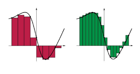
Riemann integrals of a function — Lower and upper Riemann sums

It follows that a finite number of hidden nodes can approximate any such function arbitrarily closely, since we can model rectangles with the function:

f (x) = ϕ (w (x - b))

Indeed, this function takes on value $\frac{1}{2}$ at $x = b$ ; we can think of this as the “transition point”. The larger the value of the weight $w$ , the faster the transition from 0 to 1 happens. So if we set $b = 0$ , the transition from 0 to 1 happens at $x = 0$ . At this point, the derivative of $f$ if $w / 4$ , to the width of the transition is of the order of $4 / w$ .

All of the above says that we can create a rectangle that jumps from 0 to 1 at $x = a$ and jumps back to 0 at $x = b$ , with $a < b$ , with the following, taking a very large value for $w$ :

ϕ (w (x - a)) - ϕ (w (x - b))

A few of these rectangles are graphed below:

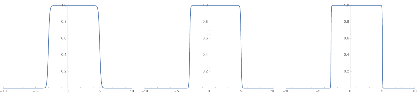
Plots of rectangles produced by different values of w — Approximate rectangles for $w = 10, 20, 50$ , respectively

This special rectangle formula has a simple representation in the form of a neural net. This network creates a rectangle from $a$ to $b$ with transition weight $w$ and height $h$ : the output of the nodes in the hidden layer is $ϕ (w (x - a))$ and $ϕ (w (x - b))$ , respectively.

A neural net implementation of the above rectangle function

Scaling this up, we can create the number of rectangles we need to do a Riemann approximation of the function.

Note that doing the Riemann integral is rarely, if ever, the best way to approximate a function. We wouldn’t want to approximate a smooth function with horrible squares. The argument here isn’t that this is an efficient approach, just that NNs are capable of doing this.

Other activation functions

The same argument also holds under other activation functions. For instance, let’s try to work it out with the rectified linear unit (ReLU) function:

(x)_{+} = max {0, x}

Let $f (x)$ be the function we’re trying to approximate. The Stone-Weierstrass theorem tells us that for every $ϵ > 0$ , there’s a polynomial $p (x)$ locally approximating it arbitrarily precisely; that is, for all $x \in [0, 1]$ , we have:

| f (x) - p (x) | < ϵ

This function $f (x)$ can also be approximated in $L_{\infty}$ norm by piecewise linear function of the form:

q (x) = m \sum i = 1 (a_{i} x + b_{i}) I_{{r_{i - 1} \leq x < r_{i}}}

Where $0 = r_{0} < r_{1} < \dots < r_{m} = 1$ is a suitable partition of $[0, 1]$ . This continuity imposes the constraint:

a_{i} r_{i} + b_{i} = a_{i + 1} r_{i} + b_{i + 1}, i = 1, \dots, m - 1

This allows us to rewrite the $q (x)$ function as follows:

q (x) = {~ a}_{1} x + {~ b}_{1} + m \sum i = 2 {~ a}_{i} (x - {~ b}_{i})_{+}

Where:

a_{1} = {~ a}_{1}, a_{i} = m \sum j = 1 {~ a}_{i}, {~ b}_{i} = r_{i - 1}

Popular activation functions

Sigmoid

The sigmoid function $σ (x)$ has a domain of $[0, 1]$ . The main problem with sigmoid is the gradient for large values of $x$ , which goes very close to zero. This is known as the “vanishing gradient problem”, which may make learning slow.

ϕ (x) = σ (x) = \frac{1}{1 + e^{- x}}

Tanh

The hyperbolic tangent has a domain of $[- 1, 1]$ . It suffers from the same “vanishing gradient problem”.

ϕ (x) = tanh (x) = \frac{e^{x} - e^{- x}}{e^{x} + e^{- x}} = 2 σ (2 x) - 1

ReLU

Rectified linear unit (ReLU) is a very popular choice, and is what works best in most cases.

ϕ (x) = (x)_{+} = max {0, x}

ReLu is always positive, and is unbounded. A nice property about it is that its derivative is 1 (and does not vanish) for positive values of $x$ It has 0 derivative for negative values, though.

Leaky ReLU

Leaky ReLu solves the 0-derivative problem of ReLU by adding a very small slope $α$ (a hyper-parameter that can be optimized) for negative values:

ϕ (x) = max {α x, x}

Maxout

Finally, maxout is a generalization of ReLU and leaky ReLU. Again, the constants can be optimized. Note that this is quite different from previous cases, where we computed the activation function of a weighted sum. Here, we compute $k \geq 2$ different weighted sums, and then choose the maximum.

ϕ (x) = max {x^{T} w_{1} + b_{1}, \dots, x^{T} w_{k} + b_{k}}

SGD and Backpropagation

Remember that the value of every node is computed by:

x_{j}^{(l)} = ϕ (K \sum i = 1 w_{i, j}^{(l)} x_{i}^{(l - 1)} + b_{j}^{(l)})

We’d like to optimize this process. Let’s assume that we want to do a regression. Let’s denote the output of the neural net by the function $f$ . Our cost function would then simply be:

L = \frac{1}{N} N \sum n = 1 (y_{n} - f (x_{n}))^{2}

We’ll omit regularization for the simplicity of our explanation, but it can trivially be added in, without loss of generality.

To optimize our cost, we’d like to do a gradient descent. Unfortunately, this problem is not convex¹³, and we expect it to have many local minima, so there is no guarantee of finding an optimal solution. But the good news is that SGD is stable when applied to a neural net, which means that the outcome won’t be too dependent on the training set. SGD is still the state-of-the art in neural nets.

Let’s do a stochastic gradient descent on a single data point. We need to compute the derivative of the cost of this single point, which is:

\frac{\partial L_{n}}{\partial w_{i, j}^{(l)}}, \frac{\partial L_{n}}{\partial b_{j}^{(l)}}

We can gain a more general formula by restating the problem in vector form. Generally, a layer of neurons is computed by:

x^{(l)} = f^{(l)} (x^{(l - 1)}) = ϕ ({(W^{(l)})}^{T} x^{(l - 1)} + b^{(l)})

The overall function of the neural net is thus something taking the input layer $x^{(0)}$ , and passing it through all hidden layers:

y = f (x^{(0)}) = f^{(L + 1)} \circ \dots \circ f^{(2)} \circ f^{(1)} (x^{(0)})

To make things more convenient, we’ll introduce notation for the linear part of the computation of a layer. The computation below corresponds to our forward pass.

\begin{matrix} z^{(l)} & = {(W^{(l)})}^{T} x^{(l - 1)} + b^{(l)} x^{(l)} & = ϕ (z^{(l)}) \end{matrix}

To be formal, we’ll just quickly state that our notation here means that we’re applying $ϕ$ component-wise. We see that to compute a $x^{(l)}$ , we need $x^{(l - 1)}$ ; we therefore need to start from the input layer and compute our way forward, until the last layer, which is why this is called the forward path.

Note that the full chain of computation that gets us to the output in $O (K^{2} L)$ , which is not too bad.

For the backwards pass, let’s remember that the cost of a single data-point is:

L_{n} = (y_{n} - f^{(L + 1)} \circ \dots \circ f^{(2)} \circ f^{(1)} (x^{(0)}))^{2}

we’ll want to compute the following, which is a derivative over both $\partial w_{i, j}^{(l)}$ and $\partial b_{j}^{(l)}$ .

\begin{matrix} δ_{j}^{(l)} & = \frac{\partial L_{n}}{\partial z_{j}^{(l)}} = \sum k \frac{\partial L_{n}}{\partial z_{k}^{(l + 1)}} \frac{\partial z_{k}^{(l + 1)}}{\partial z_{j}^{(l)}} = \sum k δ_{k}^{(l + 1)} W_{j, k}^{(l + 1)} ϕ^{'} (z_{j}^{(l)}) \end{matrix}

We can write this more compactly using $⊙$ , which is the Hadamard product (element-wise multiplication of vectors):

δ δ^{(l)} = (W^{(l + 1)} δ δ^{(l + 1)}) ⊙ ϕ^{'} (z^{(l)})

Here, to compute a $δ δ^{(l)}$ , we need $δ δ^{(l + 1)}$ ; we must therefore start from the output, and compute our way back to layer 0, which is why we call this a backwards pass. Speaking of which, we will need a $δ^{(L + 1)}$ to start with on the the right side. Therefore, we set:

δ^{(L + 1)} = - 2 (y_{n} - x^{(L + 1)}) ϕ^{'} (z^{(L + 1)})

Note that $z^{(L + 1)}$ , $δ^{(L + 1)}$ and $x^{(L + 1)}$ are denoted as scalars because we assumed that our neural net only had a single output node.

Now that we have both $z^{(l)}$ and $δ δ^{(l)}$ , let’s go back to our initial goal, which is to compute the following:

\frac{\partial L_{n}}{\partial w_{i, j}^{(l)}} = \sum k \frac{\partial L_{n}}{\partial z_{k}^{(l)}} \frac{\partial z_{k}^{(l)}}{\partial w_{i, j}^{(l)}} = \frac{\partial L_{n}}{\partial z_{k}^{(l)}} \frac{\partial z_{k}^{(l)}}{\partial w_{i, j}^{(l)}} = δ_{j}^{(l)} x_{i}^{(l - 1)}

We were able re-express this as a product of these elements that we already have. We were able to drop the sum because changing a single weight $w_{i, j}^{(l)}$ only changes the single sum $z_{j}$ ; all other sums stay unchanged, and therefore do not enter into the derivative with respect to $w_{i, j}^{(l)}$ . In other words, the term $\frac{\partial z_{k}^{(l)}}{\partial w_{i, j}^{(l)}}$ is only non-zero when $j = k$ .

We’ve thus found the result of the two derivatives we wanted to originally find:

\frac{\partial L_{n}}{\partial w_{i, j}^{(l)}} = δ_{j}^{(l)} x_{i}^{(l - 1)}, \frac{\partial L_{n}}{\partial b_{j}^{(l)}} = δ_{j}^{(l)}

Regularization

To regularize the weights, we can add $Ω (W)$ to the cost function. Typically, we don’t include bias terms in the regularization (experience shows that it just doesn’t work quite as well). Therefore, the regularization term is expressed as something like:

Ω (W) = \frac{1}{2} μ^{(l)} L + 1 \sum l = 1 {∥ ∥ W^{(l)} ∥ ∥}_{Frob}^{(l)}

We have different weights $μ^{(l)} \geq 0$ for each layer. With the right constants $μ^{(l)}$ , this regularization will favor small weights and can help us avoid overfitting.

Let $Θ = w_{i, j}^{(l)}$ denote the weight that we’re updating, and let $η$ be the step size. Assuming that we use the same weight $μ^{(l)} = μ$ for all layers $l$ , the gradient descent rule becomes:

Θ^{(t + 1)} = Θ^{(t)} - η (\nabla_{Θ} L + μ Θ^{(t)}) = Θ^{(t)} (1 - η μ) + η \nabla_{Θ} L

Usual GD deducts the step size $η$ times the gradient from the variable, but here, we also decrease the weights by a factor $(1 - η μ)$ ; we call this weight decay.

Dataset augmentation

The more data we have, the better we can train. In some instances we can generate new data from the data we are given. For instance, with the classic MNIST database of handwritten digits, we could generate new data by generating rotated characters from the existing dataset. That way, we can also train our network to become invariant to these transformations. We could also add a small amount of noise to our data (by means of compression to degree $K$ with PCA, for instance).

Dropout

We define the probability $p_{i}^{(l)}$ to be the probability of whether or not to keep node $i$ in layer $l$ in the network at a given step. A typical value would be $p_{i}^{(l)} = 0.8$ , which means 80% chance of keeping a given node. This defines a different subnetwork at every step of SGD.

There are many variations of dropout; we talked about dropping nodes, but one could also drop edges. To predict, we can generate $K$ subnets and take the average prediction. Alternatively, we could use the whole network for the prediction, but scaling the output of node $i$ at layer $l$ by $p_{i}^{(l)}$ , which guarantees that the expected input at each node stays the same as during training.

Dropout is a method to avoid overfitting, as nodes cannot “rely” on other nodes being present. It allows us to do a kind of model averaging, as there’s an exponential number of subnetworks, and we’re averaging the training over several of them. Averaging over many models is a standard ML trick, that’s usually called bagging, which usually leads to improved performance.

Convolutional nets

The basic idea in convolutions is to slide a small window (called a filter) over an array, and computing the dot product between the filter and the elements it overlaps for every position in the array. A good introduction to the subject can be found on Eli Bendersky’s website.

Structure

Classically, we’ve defined our networks as fully connected graphs, where every node in layer $l$ is connected to every node in layer $l - 1$ . This means that if we have $K$ nodes in each of the two layers, we have $K^{2}$ edges, and thus parameters, between them. Convolutional nets allow us to have somewhat more sparse networks.

In some scenarios, it makes sense that a more local processing of data should suffice. For instance, convolutions are commonly used in signal processing, were we have a discrete-time system (e.g. audio samples forming an audio stream), which is denoted by $x^{(0)} [n]$ . To process the stream we run it through a linear filter $f [n]$ , which produces an output $x^{(1)} [n]$ . This filter is often “local”, looking at a window of size $k$ around a central value:

x^{(1)} [n] = \sum k f [k] x^{(0)} [n - k]

We have the same scenario if we think of a 2D picture, where the signal is $x^{(0)} [n, m]$ . The filter can bring out various aspects, either smoothing features by averaging, or enhancing them by taking a so-called “high-pass” filter.

x^{(1)} [n, m] = \sum k, l f [k, l] x^{(0)} [n - k, m - l]

The output $x^{(1)}$ of the filter at position $[n, m]$ only depends on the values of the input $x^{(0)}$ at positions close to $[n, m]$ . This is more sparse and local than a fully connected network. This also implies that we use the same filter at every position, which drastically reduces the number of parameters.

In ML, we do something similar. We have a filter with a fixed size $K_{1} \times K_{2}$ with coefficients for every item in the filter. We move the filter over the input matrix, and compute a weighted sum for every position in the matrix.

Padding

To handle border cases, we can either do:

Zero padding, where give the filter a default value (usually 0) when going over the edges.
Valid padding, where we are careful only to run the filter within the bounds of the matrix. This results in a smaller output matrix.

Channels

A picture naturally has at least three channels: every pixel has a red, green and blue component. So a 2D picture can actually be represented as a 3D cube with a depth of 3. Each layer in the depth represents the same 2D image in red, green and blue, respectively. Each such layer is called a channel.

Channels can also stem from the convolution itself. If we’re doing a convolution on a 2D picture, we may want to use multiple filters in the same model. Each of them produces a different output; these outputs are also channels. If we produce multiple 2D outputs with multiple filters, we can stack them into a 3D cube.

As we get deeper and deeper into a CNN, we tend to add more and more channels, but the 2D size of the picture typically gets smaller and smaller, either due to valid padding or subsampling. This leads to a pyramid shaped structure, as below.

Example of a CNN getting deeper and deeper

Training

CNNs are different from fully connected neural nets in that only some of the edges are present, and in that they use weight sharing. The former makes our weight matrices sparser, but doesn’t require any changes in SGD or backpropagation; the latter requires a small modification in the backpropagation algorithm.

With CNNs, we run backpropagation ignoring that some weights are shared, considering each weight on each edge to be an independent variable. We then sum up the gradients of all edges that share the same weight, which gives us the gradient for the network with weight sharing.

Why we do this may seem a little counterintuitive at first, but we’ll attempt to give the mathematical intuition for it. Let’s consider a simple example, in which we let $f (x, y, z)$ be a function from $R^{3} \to R$ . If we let $g (x, y) = f (x, y, x)$ , then $z$ is no longer an independent variable, but is instead fixed to $z = x$ . The gradients of $g$ and $f$ are given by:

\begin{matrix} \nabla g (x, y) & = (\frac{\partial g (x, y)}{\partial x}, \frac{\partial g (x, y)}{\partial y}) \nabla f (x, y, z) & = (\frac{\partial f (x, y, z)}{\partial x}, \frac{\partial f (x, y, z)}{\partial y}, \frac{\partial f (x, y, z)}{\partial z}) \end{matrix}

To compute the gradient of $g$ , we can first compute that of $f$ , and then realize that:

(\frac{\partial g (x, y)}{\partial x}, \frac{\partial g (x, y)}{\partial y}) = (\frac{\partial f (x, y, z)}{\partial x} + \frac{\partial f (x, y, z)}{\partial z}, \frac{\partial f (x, y, z)}{\partial y})

This is a general property: we can add up the derivatives of the shared weights to compute the value of a single derivative.

Bayes Nets

We’ve often seen in this course that there are multiple ways of thinking of the same things; for instance, we’ve often seen different models as variations of least squares, and seen different ways of getting back to least squares (e.g. the probabilistic approach assuming linear model with Gaussian noise, in which we maximize likelihood, or the approach in which we try to minimize MSE, etc).

But these have often been based on very simple assumptions. To model more complex models of causality, we turn to graphical models. They allow to use a graphical depiction of the relationships between random variables. The most prominent ones are Bayes Nets, Markov Random Fields and Factor Graphs.

From distribution to graphs

Assume that we’re given a large set of random variables $X_{1}, \dots, X_{D}$ and that we’re interested in their relationships (e.g. whether $X_{1}$ and $X_{2}$ are independent given $X_{3}$ ). It doesn’t matter if these are discrete or continuous; we’ll just think of them as being discrete, and consider $p (\cdot)$ to be the density.

The most generic way to write down this model is to write it as a generic distribution over a vector of random variables. The chain rule tells us:

p (X_{1}, \dots, X_{D}) = p (X_{1}) p (X_{2} ∣ X_{1}) \dots p (X_{D} ∣ X_{1}, \dots, X_{D - 1})

In the above, we used the natural ordering $X_{1}, X_{2}, \dots, X_{D}$ , but we could just as well have used any of the $D!$ orders: this degree of freedom will be important later. Each variable in this chain rule formulation is conditioned on other variables. For instance, for $D = 4$ , we have:

p (X_{1}, X_{2}, X_{3}, X_{4}) = p (X_{1}) p (X_{2} ∣ X_{1}) p (X_{3} ∣ X_{1}, X_{2}) p (X_{4} ∣ X_{1}, X_{2}, X_{3})

A way to represent this expansion of the chain rule is to draw which variables are conditioned on which. In Bayes nets, we draw an arrow from each variable to the variables that are conditioned on it.

The Bayes net corresponding to the above

It’s important not to interpret this as causality, because the ordering that we picked chain rule is arbitrary, and could lead to many kind of arrows in the Bayes nets representation. If we just have $D = 2$ , we could have an arrow from $X_{1}$ to $X_{2}$ just as well as the other way around. The arrows are sufficient condition to guarantee dependence, but not a necessary one: they allow for dependence, but don’t guarantee it.

Still, when we know that two variables are (conditionally) independent, we can remove edges from the graph. Perhaps we have $p (X_{3} ∣ X_{1}, X_{2}) = p (X_{3} ∣ X_{2})$ , in which case we can draw the same graph, but without the edge from $X_{1}$ to $X_{3}$ .

The Bayes net where X1 is independent from X3 conditional on X2

This is suddenly much more interesting. Allowing to remove edges between independent variables means that we can have many different graphs. If we couldn’t do that, we would always generate the same graph with the chain rule, in the sense that it would always have the same topology; the exact ordering could still change depending on how we apply the chain rule. This is what will allow us to get information on independence from a graph.

Cyclic graphs

Bayes net with a cycle

The above net would correspond to the factorization:

p (X_{1} ∣ X_{2}) p (X_{2} ∣ X_{3}) p (X_{3} ∣ X_{1})

This is clearly not something that could stem from the chain rule, and therefore, the graph is not valid. In fact, we can state a stronger assertion:

Valid Bayes nets are always DAGs (directed acyclic graphs). There exists a valid distribution (a valid chain rule factorization) iff there are no cycles in the graph.

Conditional independence

Now, assume that we are given an acyclic graph. We’d like to find an appropriate ordering in the chain rule in order to find the distribution. A few things to note before we start:

Every acyclic graph has at least one source, that is, a node that has no incoming edges
Two random variables $X$ and $Y$ are independent if $p (X, Y) = p (X) p (Y)$
$X$ is independent of $Y$ given $Z$ (which we denote by $X ⊥ Y ∣ Z$ ) if $p (X, Y ∣ Z) = p (X ∣ Z) p (Y ∣ Z)$
When we talk about path in the following, we mean an undirected path

Let’s look at some simple graphs involving three variables, which will help us clarify the concept of D-separation. We’ll always ask the two same questions:

Is $X_{1} ⊥ X_{2}$ ?
Is $X_{1} ⊥ X_{2} ∣ X_{3}$ ?

These examples have names describing whether we’re comparing the head (source) or tail (sink) of the graph when asking about (conditional) independence of $X_{1}$ and $X_{2}$ .

Tail-to-tail

$X_{3}$ is the source of this graph, so the factorization is:

p (X_{1}, X_{2}, X_{3}) = p (X_{3}) p (X_{1} ∣ X_{3}) p (X_{2} ∣ X_{3})

Intuitively, $X_{1}$ and $X_{2}$ are not independent here, as $X_{3}$ influences them both; it would be easy to construct something where they are both correlated (e.g. if we let them be fully dictated by $X_{3}$ ).

To know if they are conditionally independent, let’s look at the conditioned quantity $p (X_{1}, X_{2} ∣ X_{3})$ :

\begin{matrix} p (X_{1}, X_{2} ∣ X_{3}) & = \frac{p (X_{1}, X_{2}, X_{3})}{p (X_{3})} = \frac{p (X_{3}) p (X_{1} ∣ X_{3}) p (X_{2} ∣ X_{3})}{p (X_{3})} = p (X_{1} ∣ X_{3}) p (X_{2} ∣ X_{3}) \end{matrix}

This proves $X_{1} ⊥ X_{2} ∣ X_{3}$ .

Let’s try to look at it in more general terms. We have a path between $X_{1}$ and $X_{2}$ , which in general is worrisome as it may indicate some kind of relationship. But if we know what the value of $X_{3}$ is, then the knowledge of $X_{3}$ “blocks” that dependence.

Head-to-tail

$X_{1}$ is the source of the graph, so the factorization is:

p (X_{1}, X_{2}, X_{3}) = p (X_{1}) p (X_{3} ∣ X_{1}) p (X_{2} ∣ X_{3})

We can clearly construct a case where $X_{1}$ and $X_{2}$ are dependent (e.g. if we pick $X_{1} = X_{3} = X_{2}$ ). So again, $X_{1}$ and $X_{2}$ are not independent.

To know if they are conditionally independent, let’s look at the conditioned quantity $p (X_{1}, X_{2} ∣ X_{3})$ :

\begin{matrix} p (X_{1}, X_{2} ∣ X_{3}) & = \frac{p (X_{1}, X_{2}, X_{3})}{p (X_{3})} = \frac{p (X_{1}) p (X_{3} ∣ X_{1}) p (X_{2} ∣ X_{3})}{p (X_{3})} = \frac{p (X_{1}) p (X_{3}) p (X_{1} ∣ X_{3}) p (X_{2} ∣ X_{3})}{p (X_{1}) p (X_{3})} = p (X_{1} ∣ X_{3}) p (X_{2} ∣ X_{3}) \end{matrix}

This proves $X_{1} ⊥ X_{2} ∣ X_{3}$ . Again, conditioned on $X_{3}$ we block the path from $X_{1}$ to $X_{2}$ .

Head-to-head

Here, $X_{3}$ is the source of the graph, and the factorization is:

p (X_{1}, X_{2}, X_{3}) = p (X_{1}) p (X_{2}) p (X_{3} ∣ X_{1}, X_{2})

In this example, $X_{1}$ and $X_{2}$ are independent. But if we condition on $X_{3}$ , they become dependent. So contrary, to the two previous cases, conditioning on $X_{3}$ creates a dependence. This phenomenon is called explaining away.

D-separation

Instead of determining independence manually as we did above, we can use the two following criteria to decide on (conditional) independence graphically. We’ll give a series of nested definitions that will eventually lead to the criteria. Note that these definitions talk about sets of random variables, but this also applies to single random variables (which we can consider as a set of one).

Let $X$ , $Y$ and $Z$ be sets of random variables. $X ⊥ Y ∣ Z$ if $X$ and $Y$ are D-separated by $Z$ .
We say that $X$ and $Y$ are D-separated by $Z$ iff every path from any element of $X$ to any element of $Y$ is blocked by $Z$ .
We say that a path from node $X$ to node $Y$ is blocked by $Z$ iff it contains a variable $U$ such that either:
- $U$ is in $Z$ and is head-to-tail
- $U$ is in $Z$ and is tail-to-tail
- The node is head-to-head and neither this node nor any of its descendants are in $Z$

Descendant means that there exist a directed path from parent to descendant.

Examples

Let’s do lots of examples to make sure that we understand this. We’ll be working on the following graph, and ask about different combinations of random variables.

Example of a Bayes net containing all 3 kinds of relationship

Is $X_{1} ⊥ X_{3} ∣ X_{2}$ ?

First, let’s try to understand the idea of paths. There is only one path between $X_{1}$ and $X_{3}$ : from $X_{1}$ to $X_{2}$ to $X_{3}$ . In general, it doesn’t have to be a directed path, although this one happens to be so.

For every such path—and in this case, there is just one, so it’s easy—, we’ll check if it contains is a variable that is head-tail in $Z = {X_{2}}$ . This is the case, and $X_{2}$ is head-to-tails with respect to this path. This means that the only path is blocked by $X_{2}$ , and therefore that $X_{1} ⊥ X_{3} ∣ X_{2}$ .
Is $X_{3} ⊥ X_{1} ∣ X_{2}$ ?

This is the same as above, except that the independence is stated in reverse. We know that independence is commutative, and it also follows from the D-separation lemma, since paths are not directed.
Is $X_{4} ⊥ X_{1} ∣ X_{2}$ ?

There’s only one path from $X_{4}$ to $X_{1}$ . We’ll check if it contains a variable $U \in Z = {X_{2}}$ : the only node that fits this is quite trivially $U = X_{2}$ , which is head-to-tail with respect to the path. It therefore blocks the path, and we have $X_{4} ⊥ X_{1} ∣ X_{2}$ .
Is $X_{4} ⊥ X_{1} ∣ X_{3}$ ?

There’s only one path from $X_{4}$ to $X_{1}$ , and it doesn’t contain any head-to-tail or tail-to-tail nodes in $Z$ . It does however contain a head-to-head node, $X_{3}$ . While $X_{3}$ has no descendants, we still have $X_{3} \in Z = {X_{3}}$ , and therefore, the lemma does not apply. The answer is therefore no.
Is $X_{4} ⊥ X_{1} ∣ X_{3}, X_{2}$ ?

In this case, we have $Z = {X_{2}, X_{3}}$ . There’s still only one path from $X_{4}$ to $X_{1}$ . We saw previously that we cannot apply the lemma with $X_{3}$ , so let’s try with $X_{2}$ : this node is head-to-tail with respect to the path, and belongs to $Z$ . Therefore, $X_{2}$ blocks the path, and we have a D-separation, which means that the answer is yes.
Is $X_{4} ⊥ X_{1}$ ?

There’s only one path between them, which is blocked by $X_{3}$ which is head-to-head, and $X_{3} \notin Z = \emptyset$ , and it has no descendants (so none of them are in $Z$ ). Therefore, the answer is yes.

Markov blankets

Given a node $X_{i}$ , we can ask if there is a minimal set so that every random variable outside this set is conditionally independent of $X_{i}$ . The answer to this is the Markov blanket.

The Markov blanket of $X_{1}$ is the set of parents, children, and co-parents of $X_{i}$ . By co-parent, we mean other parents of the children of $X_{i}$ .

Example of a Markov blanket — The Markov blanket of $X_{1}$ is colored in gray

Sampling and marginalizing

So far we’ve seen how to recognize independence relationships from a Bayes net. Another possible task is to sample given a Bayes net, or to compute marginals from a Bayes net. As it turns out, these two tasks are related.

First, let’s assume we know how to sample from a Bayes net. Let’s assume that we have a set of $D$ binary random variables, $X_{i} \in {0, 1}$ . We can then generate $N$ independent samples ${x_{n}}_{n}^{N} = {(X_{1 n}, \dots, X_{D n})}_{1 n}^{N}$ . To get the marginal for $X_{i}$ , we estimate $E [X_{i}]$ by computing the empirical quantity $\frac{1}{N} \sum_{n = 1}^{N} x_{i n}$ . As $N \to \infty$ , we know that this converges to the true mean.

Conversely, assume we know how to efficiently compute marginals from any Bayes net, and that we’d like to sample from the joint distribution. We can then compute the marginal of the net with respect to a certain variable $X_{i}$ , and then flip a coin according to the marginal probability we’ve computed.

The problem is that neither of these can be done efficiently, except for some special cases. The chain rule tells us that $X_{i}$ is conditioned on $X_{1}, \dots, X_{i - 1}$ , which means we’d need to have a table of $2^{i - 1}$ conditional probabilities. In general, the storage requirement is exponential in the largest number of parents any node in the Bayes net has.

Factor graphs

Assume we have a function $f$ that can be factorized as follows:

f (X_{1}, X_{2}, X_{3}, X_{4}) = f_{a} (X_{1}) f_{b} (X_{2}, X_{3}) f_{c} (X_{3}, X_{4})

A very natural representation is another graphical representation. Each variable $X_{i}$ gets a node, and each factor $f_{j}$ gets a factor node.

Factor graph of the above function

If the factor graph is a bipartite tree (i.e. no cycles), then we can marginalize very efficiently with a message-passing algorithm, which runs in linear time in the number of edges, instead of exponential complexity in the size of the network.

Sadly, very few probability distributions do us the favor of producing a tree in the factor graph. But it turns out that there many probability distributions where the factorization’s terms are fairly small, and despite cycles in the graph, we can still run the algorithm and it works approximately.

I’ve done my best to respect this notational convention everywhere in these notes, but a few mistakes may have slipped through. If you see any, please correct me in the comments below! ↩
To understand why, see the sections on optimality conditions and on single parameter linear regressions ↩
We accept this without a formal proof for now, but it should be clear from the section on convexity that MSE is convex. Otherwise, the section on normal equations for multi-parameter linear regression has more complete proofs. ↩
Convergence in probability means that the actual realizations of $X$ converges to that of $Y$ (i.e. $P (X = Y) \to 1$ ), while convergence in distribution means that the distribution function of $X$ converges to that of $Y$ (but without any guarantee that the actual realizations will be the same). Convergence in probability implies convergence in distribution, and is therefore a stronger assertion. ↩ ↩²
Fisher information is a way of measuring the information that a random variable carries about an unknown parameter. See the Wikipedia article for Fisher information. ↩
We say “data subset” here, because, as we’ll see later, the data available to the learning algorithm $A$ is often a subset of the whole dataset, called the training set. In this subsection, $S$ actually corresponds to $S_{train}$ . ↩
Because this function squeezes inputs in $(- \infty, \infty)$ into a true probability in $[0, 1]$ , I like the name “squishification function” that 3Blue1Brown uses, but other people also call it a “squashing” function. ↩
Note that this function applies the exponential function to rather large values, so we should be careful when implementing this. ↩
We have only studied binary logistic regression, which is the basic form of logistic regression. Generalized linear models will lead us to more complex extensions, such as multinomial logistic regression. ↩
The word that expresses this idea is isotropic, meaning “uniform in all directions”. ↩
Usually, the data matrix is $N \times D$ , but here, we define it as the transpose, a $D \times N$ matrix. Don’t ask me why, because I have no clue 🤷‍♂️ ↩
The columns of an orthonormal matrix are orthogonal and unitary (they have have norm 1). The transpose is equal to the inverse, meaning that if $U$ is orthogonal, then $U^{T} U = {U U}^{T} = I$ ↩
The cost function is no longer convex as $f$ is now a forward pass through a neural net, including multiple applications of the non-linear activation function ↩

View the edit history

« Back

Linear regression

Simple linear regression

Multiple linear regression

The D>N problem

Cost functions

Properties

Good cost functions

MSE

MAE

Convexity

Optimization

Learning / Estimation / Fitting

Grid search

Optimization landscapes

Local minimum

Global minimum

Strict minimum

Smooth (differentiable) optimization

Gradient

Gradient descent

Gradient descent for linear MSE

Stochastic gradient descent (SGD)

Mini-batch SGD

Non-smooth (non-differentiable) optimization

Subgradients

Subgradient descent

Stochastic subgradient descent

Comparison

Constrained optimization

Convex sets

Projected gradient descent

Turning constrained problems into unconstrained problems

Implementation issues in gradient methods

Stopping criteria

Optimality

Step size

Least squares

Normal equations

Single parameter linear regression

Multiple parameter linear regression

Simplest way

Directly verify the definition

Compute the Hessian

Geometric interpretation

Closed form

Invertibility and uniqueness

Maximum likelihood

Gaussian distribution

A probabilistic model for least squares

Defining cost with log-likelihood

Maximum likelihood estimator (MLE)

Properties of MLE

Overfitting and underfitting

Underfitting with linear models

Extended feature vectors

Reducing overfitting

Regularization

L2-Regularization: Ridge Regression

Ridge regression

Ridge regression to fight ill-conditioning

L1-Regularization: The Lasso

Model selection

Probabilistic setup

Training Error vs. Generalization Error

Splitting the data

Generalization error vs test error

Method and criteria for model selection

Grid search on hyperparameters

Model selection based on test error

Cross-validation

Bias-Variance decomposition

Data generation model

Error Decomposition

Interpretation of the decomposition

Classification

Linear classifier

Is classification a special case of regression?

Nearest neighbor

Linear decision boundaries

Optimal classification for a known generating model

The $D > N$ problem

$L_{2}$ -Regularization: Ridge Regression

$L_{1}$ -Regularization: The Lasso