CS-323 Operating Systems
- Intro
- Processes
- Application multithreading and synchronization
- Memory management
- Demand Paging
- File Systems
- Alternative storage media
- Virtual Machines
Intro
A little bit of history
In the early, early days, users would program the raw machine. The first “abstractions” were libraries for scientific functions (sin, cos, …), and libraries for doing I/O (at the time, considered a major improvement; it was an extra card deck that you’d put behind yours). And indeed, I/O libraries are the first pieces of an OS.
In the early days, only one program would run at a time. Computers were expensive, so to get more use of the resources, we started doing multiprogramming; this just means that multiple programs are in memory at once.
What does the OS do?
- It provides abstraction, and makes the hardware easier to use. It serves as an interface between hardware and user-defined programs. In hardware, we have CPU, memory, disks and devices. The OS abstracts to processes, memory locations, files, virtual devices.
- It does resource management: it allocates hardware resources (memory, CPU) between programs and users, to make sure that they can all use the resources fairly and independently (not corrupting each other’s memory for instance)
Where does the OS live?
The CPU always operates in dual mode: there’s the kernel mode and the user mode. In terms of hardware, there’s a bit that tells you which mode you are in. In short, kernel mode is the God-mode, and user-mode is very restricted.
In kernel mode, there are additional, privileged instructions: for instance, the instruction to set the mode bit is only available in kernel mode. In this mode, you have direct access to all of memory and to devices. In user mode, you don’t actually have direct access to the disk; you can ask the kernel to write something for you (the OS is the only entity that can write to a device).
The OS runs in kernel mode, and applications run in user mode. This allows the OS to protect itself, and to solely manage applications and devices.
OS interfaces
System calls
Switching from kernel mode to user mode is easy; in kernel mode, we can simply change the mode bit and give control to the user program. The other way is more tricky; to go from user to kernel mode, a device generates an interrupt, or a program executes a trap or a system call. For that purpose, there’s a system call interface that allows the kernel and user entities to communicate. This interface is essential to the integrity of the OS. System calls include process management, memory management, file systems, device management, etc.
Traditionally, system calls went through interrupts with a number; more recently, ISAs provide dedicated instructions (you put the system call number in register %eax, then execute system call instruction. If you need more space for parameters, you can put them in registers, or use registers as pointers etc). That being said, in practice, the universally used solution is the kernel API, which is an interface to the system call interface (i.e. nobody writes system calls by hand, the library takes care of putting the appropriate data in the appropriate registers, and doing the syscalls).
Side note: Meltdown and Spectre were about some of the things in kernel space being visible in user space.
Side note: when doing a printf, we’re not writing a printf kernel call directly. First of all, there’s no kernel call code specifically for print: the console is considered to be a device that the kernel can write to. Second, we’re using the language library (called libc for C) as an additional abstraction over the kernel API (see source for printf). Note that libc makes system calls look like a function call (deliberately) but it is not just a regular function call: it’s also a user-kernel transition from one program (user) to another (kernel). This is a much more expensive operation.
Traps
A trap is generated by the CPU as a result of an error (divide by zero, privileged instruction execution in user mode, illegal access to memory, …). Generally, the result is that God (the kernel) sees this and punishes you (kills the process). Still, this works like an “involuntary” system call. It sets the mode to the kernel mode and lets it do its job.
Interrupts
Generated by a device that needs attention (packet arrived from network, disk IO completed, …). It’s identified by an interrupt number which, roughly speaking, identifies the device.
OS control flow
The OS is an event-driven program. In other words, if there’s nothing to do, it does nothing. If there’s an interrupt, a system call or an interrupt, it starts running.
The (simplified) execution flow is as follows:
- The user executes a system call or a trap with code i, or there’s an interrupt with code
i. - The hardware receives this, puts the machine in kernel mode, and depending on what it’s received, does the following:
- System call: put the machine in kernel mode, set
PC = SystemCallVector[i] - Trap: put the machine in kernel mode, set
PC = TrapVector[i] - Interrupt: put the machine in kernel mode, set
PC = InterruptVector[i]
- System call: put the machine in kernel mode, set
- The kernel executes system call
ihandler routine (after checking that theiparameter is valid), and then executes a “return from kernel” instruction - The hardware puts the machine back in user mode
- The user executes the next instruction after the system call.
OS design goals
- Correct abstractions
- Performance
- Portability: You cannot do this completely, but you can try to minimize the architecture-independent sections so that you only have to rewrite those to port to a new system.
- Reliability: The OS must never fail. It must carefully check inbound parameters. For instance, the inbound address parameter must be valid.
High-level OS structure
The simplest OS structure is the “monolithic OS”, where there’s a hard line between the whole OS, in kernel mode, and the user programs, in user mode. But the OS is a huge piece of software (millions of lines of code), so if something goes wrong in kernel mode, the machine will likely halt or crash.
Luckily, many pieces of the OS can be in user mode, and the above is a strong incentive to put them there. Indeed, some parts of the OS don’t need the privileged access, and we save some effort that way. A good example of those are daemons (printer daemon, system log, etc.), that are placed in user mode. This is known as the “systems programs” structure.
Bringing this idea to the extreme, we have the microkernel. The idea is to place the absolute minimum in kernel mode, and all the rest in user mode. This does not only place deamons in user mode, but also process management, memory management, the file system, etc. Note that these still communicate with the microkernel, but run the majority of their code in user mode. In practice, microkernels have been a commercial failure, and the “systems programs” has won out.
Processes
What is a process?
A process is a program in execution: a program is executable code on a file on disk, and when it runs, it’s a process. A process can do just about anything, as far as the user is concerned (shell, compiler, editor, browser, etc). Each process has a unique process identifier, the pid.
Basic operations on a process:
- Create
- Terminate
- Normal exit
- Error (trap)
- Terminated by another process (
KILLSIG)
Linux has a simple yet powerful list of process primitives:
fork(): if a process runs a fork, it becomes the parent of the new process. The new process is an identical copy of the process that called fork, except for one thing: in the parent, the call toforkreturns thepid, while in the child, it returns0.exec(filename): loads into memory the file with the given filename. Note that running this completely replaces the code that called theexec, it’s not like a function call that returns to the caller’s execution context. But it does leave the environment intact! More on that laterwait(): waits for one of the children to terminate (the basicwaitfunction waits for any child; there are more advanced versions that wait for a particular one).exit(): terminates the process (it’s a suicide)
Here’s some typical forking code:
if (pid = fork()) {
    wait();
} else {
    exec(filename);
}
fork will execute the fork, return the pid of the child in the parent, and 0 in the child. The parent therefore enters the if-statement and waits, while the child goes into the else-statement, and executes the file. We’re assuming that the C file in filename ends with an exit() (it’s inserted by the C compiler if you don’t explicitly write it), which causes the child process to terminate, and the parent process to stop waiting.
Side note: This may seem a bit strange: why would the new thread need to be a copy? Why use fork+exec instead of simply create (like Windows does)? A process is not just code, it’s environment and code. The environment includes ownership, open files and environment variables; note that it does not include registers or the heap or stack, or anything like that (that would probably be a big security issue). A call to fork doesn’t replace the environment, it only changes the code (and the registers, etc are reset). This default behavior allows us to have simple function calls, without a million arguments for environment like in Windows.
Outline of the Linux shell
forever {
    read from input
    if (logout) exit()
    if (pid = fork()) {
        wait()
    } else {
        // You can make changes to the environment
        // of the child here.
        exec(filename)
    }
}
You can manipulate the environment of the child without changing the environment of the parent by adding code where the comment is. For instance, a command shell may redirect stdin and stdout to a file before doing an exec.
Linux process tree
The first process, init runs from boot. When the user logs in, it forks and waits, and the child executes the shell (say, bash): at this stage, the child process is the shell process for the user running bash. Now, the user runs make, so the shell forks and waits, and its child executes make and exits. Now another user logs in, so the initial parent creates another child, and opens another shell (say, zsh). Note that init can create another process while waiting because it’s not really a normal process, it’s a “black magic” custom process. All of this creates a tree hierarchy of processes and their children.
Multiprocessing
As far as the OS is concerned, it either computes or does I/O. Back in the old days, in single-process systems, I/O would leave the CPU idle until it was complete. In a multiprocess system, another process can do processing in that time.
There are five stages that a multiprocessing system can be in:
- New
- Ready
- Running
- Waiting
- Terminated.
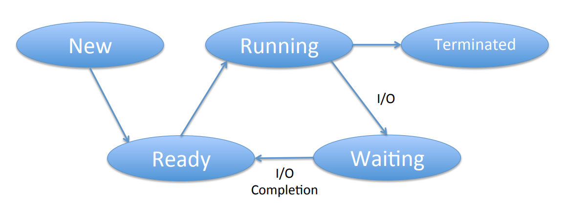
Typically, a process will start in new (1), go to ready (2), then running (3), then go to waiting to do I/O (4), then to ready (2, using an interrupt), then back to running (3, picked by the scheduler); it can loop in 2-4 an arbitrary number of times, and eventually terminates (5, leaving from the running state 3).
Process switching
A process switch is a switch from one process running on the CPU to another CPU, so that you can later switch back to the process currently holding the CPU.
This is not so simple, because a process consists of many things: the code, stack, heap, values in register (including PC) and MMU info (memory management unit, we can ignore this for now). The first three reside in process-private location, but the last two reside in shared locations. To make the swap possible, the registers are backed up to the process control block (PCB, though Linux has another name for it); in addition it contains information about the process, and some save area (free space).
A process switch is an expensive operation. It requires saving and restoring a lot of stuff, so it has to be implemented very efficiently (often written in machine code, as one of the only parts of the kernel), and has to be used with care.
Process scheduling
In general, many processes may be in the ready state. It is the scheduler’s job to pick out a process in the ready state and set it to the running state.
In practice, there’s often a timer on the running state that sets a thread back to ready after say, 10ms, if it isn’t doing IO. A scheduler that does this is called a preemptive scheduler.
In a non-preemptive scheduler, a process can monopolize the CPU, as it is only stopped when it voluntarily does so; thus a non-preemptive scheduler is only useful in special circumstances (for instance, in the computer of an airplane autopilot, where we absolutely must have the thread running at all times).
The scheduler must remember the running process, and maintain sets of queues (ready queue, I/O device queue). The PCBs sit in queues.
The scheduler runs when:
- A process starts or terminates (system call)
- The running process performs an I/O (system call)
- I/O completes (I/O interrupt)
- Timer expires (timer interrupt)
Scheduling algorithm
What makes a good scheduling algorithm? It depends.
There are two kinds of processes, that require different scheduling tactics:
- Interactive processes: the user is waiting for the result (browser, editor, …)
- Batch processes: the user will look at the result later (supercomputing center, …).
For batch, we want high throughput, meaning that we want a high number of jobs completed over say, a day. From a throughput perspective, the scheduler is overhead, so we must run it as little as possible. But for interactive applications, we want to optimize response time, so we want to go from ready to running quickly, which means running the scheduler often.
We’ll look at a few algorithms.
- FCFS (first come first served): when a process goes to ready, we insert at the tail of the queue; this way, we always run the oldest process (head of the queue). By definition, this is non-preemptive. It has low overhead, good throughput, but uneven response time (you can get stuck behind a long job), and in extreme cases, a process can monopolize the CPU.
- SJF (shortest job first): we order the queue according to job length. We always run the head of the queue, which is the shortest available job. It can be preemptive or non-preemptive, but we’ll consider the preemptive only. It has good response time for short, but can lead to starvation of long jobs, and it’s difficult to predict job length.
- RR (Round Robin): We define a time quantum x. When a process is ready, we put it at the tail (like FCFS). We run the head and run it for x time, after which we put it at the tail of the queue.
RR works as a nice compromise for long and short jobs. Short jobs finish quickly, long jobs are not postponed forever. There’s no need to know job length; we discover length by counting the number of time quantums it needs.
Application multiprocess structuring
If we wanted to build a web server, the minimal version would just wait from incoming requests, read files from disks and send the file back in response. This is pretty terrible, so we can use processes to accept other connections while we’re reading from disk, so that another process can use the CPU in the meantime, overlapping computing with IO.
Thus, the server now has a structure with a single listener, and a number of worker processes. But generating processes is expensive, especially if we have to do it for every request! Therefore, we can create what’s called a process pool: we create worker processes during initialization, and hand incoming requests to them. The structure remains the same (a listener, multiple workers), but the amount of work per request decreases, since sending a message is cheaper than creating a worker.
However, to be able to do so, we need a mechanism for interprocess communication, which is what we’ll see in the next section.
Interprocess communication
There are two key ways of doing this, and they’re somewhat related: message passing, and remote procedure call.
Message passing
This is the simplest, with only two primitives: send a message, and receive a message. Note that message passing is always by value, never by reference.
This is implemented in the kernel through a table (proctable) which, for every pid has a queue (linked list) of waiting messages for the process with pid to process; other processes can add to this queue.
There are of course more complex alternatives:
- Symmetric vs. asymmetric: in symmetric, the sender and the receiver both communicate with a specific, given process (they know each other). In asymmetric, the sender sends to a particular process, and the client receives the message from any process, and get the message + pid (to be able to reply). Asymmetric is more common.
- Blocking vs. non-blocking: for sending, non-blocking returns immediately after the message is sent, while blocking blocks until the message has been received. For receiving, non-blocking returns immediately, while blocking blocks until a message is present. For receiving, non-blocking sending is more common.
A very common pattern is:
- Client:
- Send request
- Blocking receive
- Server
- Blocking receive
- Send reply
This works somewhat like a function call, and it’s basically how remote procedure calls work.
Remote procedure call
Another possibility is to use remote procedure calls. To use these, we link a client stub with the client code, and a server stub with the server code. In other words, every code instance has an associated stub. The stubs’ job is to:
- Client code does a proc call to the client stub
- Client stub sends a message through the kernel
- Server stub receives the request from the kernel
- Server stub calls the correct code through a proc call
- Server code sends a return proc call with the return value
- Server stub replies to client stub through a message through the kernel
- Client stub returns correct value to client code through a proc call
Application multithreading and synchronization
Multithreading vs. multiprocessing
In our example about the web server, there’s still a problem: disk access is expensive. To remediate this problem, we usually use caches for recently read data. But worker 1 and worker 2 are different processes, their memory is separate, and what we’ve cached for worker 1 hasn’t been cached for worker 2, who will store a separate copy (waste of time, waste of cache).
This is exactly what multiprocessing is bad at, and multithreading is good at. If not sharing memory is the problem, then sharing memory is the solution.
A thread is just like a process, but it does not have its own heap and globals. Two threads in a process share code, globals and heap, but have separate stacks, registers and program counters (PC).
Processes provide separation, and in particular, memory separation. This is useful for things that really should remain separate, so for coarse-grain separation. Threads do not provide such separation; in particular, they share memory, so they are suitable for tighter integrations.
Pthreads
Having multiple threads reading and writing to shared data is obviously a performance advantage, but is also a problem, as it can lead to data races. Data races are a result of interleaving of the thread executions. This means that to write a multi-threaded program, a program must be correct for all interleavings. To do so, we use pthreads.
The basic approach to multithreading is to divide “work” among threads. Then you need to think of which data is shared, where it’s accessed, and put the shared data in a critical section (n.b. this sentence would give professors a heart attack, but this is a good way to think about it). Putting something in a critical section means that the processor can’t interleave a code into a critical section.
Pthreads have a few available methods:
Pthread_create(&threadid, threadcode, arg): Creates thread, returnsthreadid, runsthreadcodewith argumentarg.Pthread_exit(status): terminates the thread, optionally returns statusPthread_join(threadid, &status): waits for threadthreadidto exit, and receives status, if any.Pthread_mutex_lock(mutex): if mutex is held, block. Otherwise, acquire it and proceed.Pthread_mutex_unlock(mutex): release mutex
Synchronization
To synchronize code, we use mutex locks. A common mistake is that lines such as a += 1 aren’t atomic; in reality, it corresponds to a load into a register, an increment of said register, and a store of the register into memory. During this process, the instruction sequence may be interleaved. Note that some machines have atomic increments available.
We can use locks, but single locking inhibits parallelism. To remediate this, there are two approaches: fine-grained locking, and privatization.
Privatization is the idea of defining local variables for each thread, using them for accesses in the loop, and only access shared data after the loop; when things are being put in common, we can lock.
As an example:
ListenerThread {
    for(i=0; i<MAX_THREADS; i++) thread[i] = Pthread_create(…)
    forever {
        Receive(request)
        Pthread_mutex_lock(queuelock)
        put request in queue
        Pthread_mutex_unlock(queuelock)
    }
}

WorkerThread {
    forever {
        Pthread_mutex_lock(queuelock)
        take request out of queue
        Pthread_mutex_unlock(queuelock)
        read file from disk
        Send(reply)
    }
}
Warning: This won’t work! We need to tell worker(s) that there is something for them to do, an item in the queue for them. This is sometimes called task parallelism. Pthreads have a mechanism for this:
Pthread_cond_wait(cond, mutex): wait for a signal on cond, and release the mutexPthread_cond_signal(cond, mutex): Signal one thread waiting on cond. The signaled thread re-acquires the mutex at some point in the future. If no thread is waiting, this is a no-op. Note that the function signature isn’t actually correct (there’s no mutex parameter) but it makes it easier to explain.Pthread_cond_broadcast(cond, mutex): signal all threads waiting on cond. If no thread is waiting, it’s a no-op.
We must hold the mutex when calling any of these.
We can now fix our previous example:
ListenerThread {
    for(i=0; i<MAX_THREADS; i++) thread[i] = Pthread_create(…)
    forever {
        Receive(request)
        Pthread_mutex_lock(queuelock)
        put request in queue
        // Signal that the queue isn't empty
        Pthread_cond_signal(notempty, queuelock)
        Pthread_mutex_unlock(queuelock)
    }
}

WorkerThread {
    forever {
        Pthread_mutex_lock(queuelock)
        // Wait until there is something in the queue before taking it.
        Pthread_cond_wait(notempty, queuelock)
        take request out of queue
        Pthread_mutex_unlock(queuelock)
        read file from disk
        Send(reply)
    }
}
Still, there is a slight bug in the above; if all worker threads are busy doing something, the Pthread_cond_signal will no-op. This is important to note: if no thread is waiting, either because they’re not listening or because they’re busy, the signal is a no-op. In general, signals have no memory, and they’re forgotten if no thread is waiting. So we need an extra variable to remember them:
ListenerThread {
    for(i=0; i<MAX_THREADS; i++) thread[i] = Pthread_create(…)
    forever {
        Receive(request)
        Pthread_mutex_lock(queuelock)
        put request in queue
        avail++
        Pthread_cond_signal(notempty, queuelock)
        Pthread_mutex_unlock(queuelock)
    }
}

WorkerThread {
    forever {
        Pthread_mutex_lock(queuelock)
        while (avail <= 0) Pthread_cond_wait(notempty, queuelock)
        take request out of queue
        avail--
        Pthread_mutex_unlock(queuelock)
        read file from disk
        Send(reply)
    }
}
Note that we’re doing a while here, not if. If we used an if instead, we may have a problem. It’s important not to think of the signaler passing the mutex to the waiter. The only thing we know is that the waiter will acquire the mutex lock at some point in the future; another thread may come and steal it in the meantime, and take the item in the queue! This is subtle, and we’ll have exercises about it (week 4).
Kernel multithreading
The kernel is a server. There are requests from users (system calls, traps), and from devices (interrupts). It’s an event-driven program, waiting for one of the above to start running. In Linux, there’s one kernel thread for each user thread; this is not the case in other OSes. This is called a 1-to-1 mapping.
How does it work? The user thread makes a system call, there’s a switch to kernel mode, set the PC to the system call handler routine, the SP to the kernel stack of the kernel thread. To go back to user mode, we set the SP to the stack of the user thread, and the PC to the user thread PC, return from kernel mode, and now run in user thread.
The kernel and the user threads have different stacks; otherwise, another thread in user mode could read and modify the kernel’s stack, which would be a huge security risk.
For synchronization in the kernel, there’s a different synchronization library (not Pthreads, which is a user-level library), but otherwise, it’s in any multithreaded program. There is a notable difference though; there are also interrupts in the kernel. When a device interrupts, the PC is set to the interrupt handler, the SP to the interrupt thread stack, we run the interrupt handler.
This is not exam-stuff, but let’s talk about it anyway. The interrupts must be served quickly, we cannot block it. The solution (in Linux) is to add another set of threads (soft interrupt threads). On an interrupt, we put the request in queue for soft interrupt threads, which will do the bulk of the work.
Memory management
Goals and assumptions
For this part of the course, a few assumptions:
- We will only be concerned about processor and main memory; we do not worry about L1, L2, L3 caches and disk.
- A program must be in memory to be executed (we’ll revisit this next week).
The kernel is generally located in low physical memory (close to 0), because interrupt vectors are in low memory.
Virtual and physical address spaces
For protection, one process must not be able to read or write in the memory of another process, or of the kernel. We cannot have unprotected access: all CPU memory accesses must be checked somehow (this is done in hardware; checking errors are traps).
Additionnally, we want transparency: the programmer should not have to worry where his program is in memory, or where/what other programs in memory. With transparency, the program can be anywhere in memory, and it shouldn’t affect the behavior or code of the program.
This is why we have the abstraction of virtual address space. The virtual (or logical) address space is what the program(mer) thinks is its memory, and is generated by the CPU. Physical is where it actually resides in memory.
The piece of hardware that provides mapping from virtual-to-physical and protection is the Memory Management Unit (MMU).
The size of the virtual address space is only limited by the size of addresses that CPUs can generate; on older machines, 2^32 bytes (4GB), on newer, 64-bit machines, 2^64 (16 Exabyte!). The physical address space is limited by the physical size of the memory; nowadays, it’s in the order of a few GB.
Mapping methods and allocation
Base and bounds
The virtual memory space is a linear address space, where addresses go from 0 to MAX.
The physical memory space is a linear address space, where addresses go from BASE to BOUNDS = BASE + MAX.
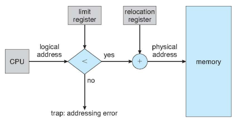
The MMU has a relocation register that holds the base value, and a limit register holding the bounds value. If a virtual address is smaller than the limit, the MMU adds the value of the relocation register to the virtual address. Otherwise, it generates a trap.
All early machines were done this way, but this is not commonly used anymore, except in very specific machines (CRAY supercomputers keep it simple to go fast).
Segmentation
With segmentation, you have multiple base and bounds within a single address space. There’s a set of segments from 0 to n, and each segment i is linear from 0 to MAX(i). A segment is whatever you want it to be. It’s a more user-centric view of memory, where each segment contains one or more units of the program (a procedure’s code, an array, …). Segmentation reduces internal fragmentation (segments are not fixed size, can be fit exactly to requirements), but can create external fragmentation (some small free memory locations may remain which never get used).
The virtual address space is two-dimensional: a segment number s, and an offset d within the segment.
The physical address space is a set of segments, each linear. The segments don’t have to be ordered like the virtual space.
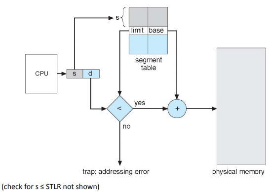
The MMU contains a STBR (Segment Table Base Register) that points to the the segment table in memory, and the STLR (Segment Table Length Register) containing the length of the segment table. The segment table is indexed by segment number, contains (base, limit) pairs where base is the physical address of the segment in memory, and limit is the length of the segment.
Segmentation is an Intel invention, but over time they’ve given it up for paging (it got programmers confused).
Paging
A page is fixed-size portion of virtual memory. A frame is a fixed-size portion of physical memory. These two are always the same size, and they have to be. A typical size these days is 4-8KB. It reduces external fragmentation (no unusable free frames, since they are all of equal size), but may increase internal fragmentation (memory is allocated in say 4KB chunks, so going over 10B into the next page wastes 4086B).
The virtual address space is linear from 0 up to a multiple of the page size. For mapping purposes, the virtual address is split into two pieces: a page number o and an offset p within that page.
The physical address space is a non-contiguous set of frames. There’s one frame per page, but not necessarily in order.
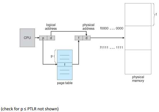
The MMU has a page table to translate page number to frame number; the offset stays the same.
Segmentation with Paging
This is a combination of the two previous methods. It looks like segmentation, but underneath it’s paged. It aims to reduce both internal and external fragmentation.
The virtual address space is exactly like segmentation: we define segments for every abstract memory group of varying sizes.
However, the physical is just like in paging (non-contiguous set of frames).
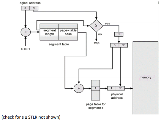
Each process keeps one segment table, and multiple page tables (one for each segment). The logical addresses are first interpreted as (segment, offset), which the segment table can translate into (page_table_number, page_number, offset), which we can give to the page table to resolve a physical address.
Optimizations
Memory allocation
How do we find memory for a newly arrived process? Base-and-bounds leaves “holes” in the memory, so we need to pick a “hole” for the new process to use. There are a few dynamic memory allocation mehtods:
- First-fit: Take the first hole that fits
- Best-fit: Take the smallest hole where we can fit what’s been requested. This sounds nice, but it also leaves small holes behind, which is problematic
- Worst-fit: takes the largest hole, and leaves big holes behind
The problem here is external fragmentation: small holes become unusable, part of memory can never be used. This is a serious problem. Main memory allocation is easier to do in segmentation. Pieces are smaller, but there are more than one. Main memory allocation is easiest in paging, as pages have a fixed size. But we now have an internal fragmentation problem: part of the last page may be unused. With a reasonable page size though, this is not too much of a problem.
Protection
Fine-grain protection means having different protections for different parts of the address space. In the page table, we can have a few bits to indicate read/write/execute rights on the memory, and whether the memory is valid. For instance, code should be valid, read-only (don’t let an attacker inject code) and executable.
In base-and-bounds, this is not really possible; we do not have any break-up, there’s no page table. In segmentation, this is easy to do: there’s a segment for the code, so we set the bits in the segment table. Same goes for paging, we can set the bits, but we have to do it in every code page.
Sharing
Sharing memory between processes allows us to run twice the same program in different processes (we can share the code), or read twice the same file in different processes (we may want to share memory corresponding to the file).
This is not possible in base and bounds. With segmentation, we create a segment for shared data, and add an entry in the segment tables of both processes pointing to shared segments in memory. With paging, this is somewhat more complex; we need to share pages, add entries in pages of both processes and point to the shared pages, and manage multiple shared pages.
Feature comparison
Segmentation is best for sharing and fine-grain protection, while paging is best for memory allocation. This is the reason we have segmentation with paging: it combines the best of both worlds and allows us to do all three fairly easily.
TLBs
For performance, we have TLBs (translation lookaside buffers), a piece of hardware outside physical memory.
They are there because the page table actually is in memory, not in a separate device as we may have been led to believe. A virtual address reference would (without the TLB) result in 2 physical memory accesses, which would reduce performance by a factor of 2. The TLB is a small fast cache of mappings (page_nb -> frame_nb). If the mapping for page_nb is found in the TLB, we use the associated value instead of looking up the page table. If not, we have to do a lookup, but we add it the mapping to the TLB.
The TLB is highly specialized, expensive hardware, but it’s also very fast. It’s an associative memory cache, meaning that there’s a hardware comparator for every entry, so the TLB is usually rather small (64-1024 entries). If it’s full, we replace existing entries.
Note that flushing the TLB is actually the real reason that process switching is so expensive (moreso than switching register values, like we said earlier). Typical TLB hit rates are 95-100%.
Dealing with large virtual address spaces
The virtual address space is 64 bits, and we’ve got 4KB pages, which means 12 bits are needed for offset, which leaves 52 bits for page number, which would require 252 page table entries. Say they’re 4 bytes each, we’d need 254 bytes (18 petabytes) of memory, which is way more than we have!
There are a few solutions to this (hierarchical page tables, hashed page tables, inverted page tables, …) but we’ll just take a look at hierarchical page tables.
The number of levels of hierarchy can vary, but here we’ll just talk about two-level page tables:
- In a single level page table, we have a set number of bits indicating the page number. In a two-level page table, we break this page number
pinto two numbersp1andp2. - The top-level page table entry is indexed by
p1, and contains a pointer to second-level page table (and a valid bit) - The second-level page table entry is indexed by
p2, and contains a frame number containing page(p1, p2)(and a valid bit)
This is useful because most address spaces are sparsely populated: As we said above, the virtual address space is very large (say, 252 pages), and we won’t be using most virtual pages. But still, in a one-level page table we need an entry for every page. Therefore, most entries in the page table will be empty (in reality, they’re not empty, just invalid: the valid bit will be 0).
We can solve this with hierarchical page tables. The first layer needs 2p1 entries (one for every possible value of the first part of the page number), but we only need second-level page tables for the populated parts of the first level. For every invalid entry in the first level, we can save ourselves 2p2 bytes, since we don’t need a level two for that.
Note that hierarchical page tables are counter-productive for dense address spaces, but since most address spaces are quite sparse, it’s usually worth it. The price to be paid here is that each level adds another memory access; instead of 1 memory access, we’ll have n+1. But the TLB still works, so if this is rare (i.e. TLB hit rate 99%), we can live with it!
Process switching and memory management
One solution, is to invalidate all TLB entries on process switch. This makes the process switch expensive!
The other solution is to have the process identifier in TLB entries, so that a match is a match on both pid and pageno. The process switch is now much cheaper; although this makes the TLB more complicated and expensive, all modern machines have this feature.
Demand Paging
We’re now going to drop the assumption that all of a program must be in memory. Typically, part of program is in memory, and all of it is on disk.
Remember: the CPU can only directly access memory. It cannot acess data on disk directly, it must go through the OS to do IO.
But what if the program acesses a part of the program that’s only on disk? The program will be suspended, the OS is run to get the page from disk, and the program is restarted. This is called a page fault, and what the OS does in response is page fault handling.
To discover the page fault, we use the valid bit in the page table. Without demand paging, if it’s 1, the page is valid, otherwise it’s invalid. With demand paging:
- If the valid bit is 0: the page is invalid or the page is on disk
- If the valid bit is 1: the page is valid and it’s in memory
Sidenote: there’s also an additional table to see invalid, on-disk pages.
Access to an invalid bit generates a trap. The OS allocates a free frame to the process, finds the page on disk, gets the disk to transfer the page from disk to this allocated frame. While the disk is busy, we can invoke the scheduler to run another process; when the disk interrupt comes in, we go back to the page fault handling, which updates the page table, and sets the valid bit to 1, gives control back to the process, restarting the previously faulting instruction which will now find a valid bit in the page table.
Page replacement
If no free frame is available for the disk to fill up, we must pick a frame to be replaced, replace its page table and TLB entry (maybe even writeback if it has a modified bit). Picking the correct page to replace is very important for performance: a normal memory access is 1ns, a page fault is 10ms. In general, we prefer replacing clean over dirty (one disk IO vs two, because we can save a writeback by picking the clean).
There are many replacement policies:
- Random: easy to implement, performs poorly
- FIFO: oldest page (brought in the earliest) is replaced. This is very easy to implement with a queue of pages, but performs pretty badly.
- OPT: replace the page that will be referenced furthest in the future. This sounds fantastic and perfect, and it is: it’s an optimal algorithm, but we can’t actually implement this, because we can’t predict the future. We just use it as a basis for comparison.
- LRU: replace least recently accessed page. This is not the same as FIFO, which looks at when a page was brought in (vs. when it was used for LRU). LRU is difficult to implement perfectly: we’d need to timestamp every memory reference, which would be too expensive. But we can approximate it fairly well with a single reference bit: periodically, we read out and store all reference bits (those are bits set by the hardware when a page is referenced), and reset them all to 0. We keep all the reference bits of the last few periods; the more periods kept, the better the approximation. We replace the page with the smallest value of reference bit history (i.e. the one last referenced the furthest back).
- Second-chance: also called FIFO with second-chance. When we bring in a page, we place it at the tail of the queue, as with FIFO. To replace, instead of taking the head page invariably as with FIFO, we give it a second chance if its reference bit is 1 (if it’s 0, no second chances, replace it). A second chance means that we put it at the tail of the queue, set the reference bit to 0, and look at the head of the queue to see if we should replace that or give it a second chance (this happens in a loop until we can replace). This works, as it is a combination of FIFO and the LRU approximation with one reference bit
- Clock: this is a variation of second chance. Imagine all the pages arranged around a (one-armed) clock. For the replacement, we look at the page where the hand of the clock is; if the bit is 0, we replace it, but if it is 1, we set it to 0 and move the hand of the clock to the next page. This is actually exactly the same as FIFO+second-chance; the clock points to the head of the queue. But clock is more efficiently implemented (Microsoft’s code is closed source, but rumor goes that it’s quite close to a clock).
In addition to the replacement algorithm, you can pick varying replacement scopes:
- Local replacement replaces a page of the faulting process. You cannot affect someone else’s working set (a term well define below), but it’s very inflexible for yourself, since you can’t grow (you cause yourself to thrash)
- Global replacement replaces any page (e.g. for FIFO, local replaces the oldest page of the faulting page, while global picks the oldest page overall). This can allow for DDOS-like attacks where one process takes over the whole memory, causing everyone else to thrash.
It’s difficult to say which one is better; in a way, there’s a tradeoff to pick from. If you’re an OS writer, though, you have to favor security before performance, so you have to favor local replacement. In reality, most OSes find some middle ground: you use frame allocation periodically (see below), with local replacement in-between. You may thrash for a short amount of time, but at the next period you’ll probably get the bigger allocation, so that’s fine. You can’t cause thrashing of others, so that’s fine too.
Frame allocation
There’s a close link between the degree of multiprocessing and the page fault rate. We can decide to:
- Give each process frames for all of its pages: this implies low multiprocessing, few page faults, slow switching on I/O
- Give each process 1 frame: high multiprocessing, many page faults (thrashing) and quick switching on I/O).
Where is the correct tradeoff between these two extremes?
To answer this, we need to know about the working set of a process: it’s the set of pages that a process will need for execution over the next execution interval. The intuition is that if the working set isn’t in memory, there will be many page faults; if it is, there will be none. There’s nothing to be gained by putting anything more than the working set in memory.
If you could somehow give each process its working set, we would have a good tradeoff between few page faults and moderate degree of multiprocessing. Why use the working set instead of all pages? It’s the principle of locality: at any given time, a process only accesses part of its pages (initialization, main, termination, error, …).
The frame allocation policy must then be able to give each process enough frames to maintain its working set in memory. If there’s no space in memory for all working sets, we need to swap out one or more processes; if there’s space, we can swap one in.
The obvious question now is how we can predict a working set: in practice, what people do is to assume that it’ll be the same as before. The working set for the next 10k references will be the same as for the last 10k references. This prediction isn’t perfect, because a program may change state (i.e. initialization to main); this will temporarily cause a high page fault rate, but then it’ll work well again.
So how do we measure the past working set? Well, we don’t really need the working set, we only need its size. Periodically, we count the reference bits set to 1, and them reset them all to 0. The working set is thus the number of reference bits set to 1.
N.B.: Frame allocation is done periodically, while page replacement is done at page fault time.
Optimizations
Prepaging
So far we’ve been paging in one page at a time. Prepaging takes multiple pages at a time. This works because of locality of virtual memory access: nearby pages are often accessed soon after. This avoids future page faults, process switches, and also allows for better disk performance (more on that later), but may bring in unnecessary pages.
Cleaning
So far, we’ve preferred to replace clean pages. Cleaning is about writing out dirty pages when the disk is idle, so that we have more clean pages at replacement time. The drawback is that the page may be modified again, which may create useless disk traffic. Still, cleaning is usually always a gain, so pretty much all systems do it periodically.
Free frame pool
So far, we used all possible frames for pages. With a free frame pool, we keep some frames unused. This makes page fault handling quick by offsetting replacement to outside page fault time. The drawback is that this reduces effective main memory size.
Copy-on-write
This is a clever trick to share pages between the processes that:
- Are initially the same
- Are likely to be read-only (remain the same)
- But may be modified in the future (although unlikely)
To understand how this works, let’s remind ourselves how read-only sharing works: we make the page table entries point to same frame, set the read-only bit so that it generates a trap if the process writes; the trap is treated as an illegal memory access.
We can’t do that in our case, because we will allow the unlikely write. Instead, when we receive the trap, we create a separate frame for the faulting process, insert the (pageno, frameno) in the page table, set the read-only bit to off (allowing read-write) and copy that page into that frame: further accesses won’t page fault.
This works well if the page is rarely written, and allows us to save sharers - 1 frames. Obviously, if the page is written often, as it causes more page faults without gaining in frame occupations. In practice though, this works very well and all OSes provide it. Linux implements fork() this way: we don’t copy the page straight away, we just wait for the new process’ first modification to copy the page.
File Systems
What is a file system?
The file system provides permanent storage. How permanent is permanent? For this course, it’ll just mean across machine failures and restarts (this is a stronger guarantee than across program invocations, but less strong than across disk failures or data center failures).
Main memory is obviously not suitable for permanent storage. In this course, we’ll only talk about disks and flash (although other technologies exist, such as tape, or battery-backed memory).
There’s no universally accepted definition of what a file is, but we’ll say the following: it’s an un-interpreted collection of objects surviving machine restarts. Un-interpreted means that the file system doesn’t know what the data means, only the application does. These objects can be different things for different OSes; in Linux, they are simple bytes (this is more common, and we’ll only talk about this), but other OSes see them as records.
Should a file be typed or untyped? Typed means that the file system (FS) knows what the object means. This is useful, because it allows us to invoke certain programs by default, prevent errors, and perhaps even store the file more efficiently on disk. However, it can be inflexible, as it may require typecasts, and for the OS, it would involve a lot of code for each type.
We will look at untyped files, which is how Linux works (but Windows uses a typed system). Note that file filename extensions (.sh, .html, …) aren’t types: in Linux, it’s pure convention. The user knows, but the system doesn’t do anything with it. In Windows, the user knows, and the system knows and enforces the type.
Interface
Access primitives
The main access primitives to the file system are:
uid = create(...): creates a new file and returns auid, a non human-readable unique identifierdelete(uid): deletes the file with the givenuidread(uid, buffer, from, to): read from file withuid, from bytefromto a byteto(this may cause an EOF condition) into a memory buffer (previously allocated, must be of sufficient size)write(uid, buffer, from, to): write to file withuidfrom bytefromto bytetofrom a memory buffer
The above read and write are random access primitives: there’s no connection between two successive accesses. This is opposed to sequential access, which reads from where we stopped reading last time, and writes to where we stopped writing last time.
In a sequential read, the file system keeps a file pointer fp (initially 0), and to execute read(uid, buffer, bytes), reads bytes bytes into buffer and increments fp by bytes.
Note that sequential could be built on top of random access; all it takes is maintaining to the file pointer. Sequential access is essentially a convenience, where the FS manages the file pointer. We can also build random access on top of sequential access thanks to the seek(uid, from) primitive, which allows us to move to a certain location in the file.
Since sequential access is more common, and managing the file pointer manually leads to many errors, Linux offers sequential access with the addition of the seek primitive to enable random access.
Concurrency primitives
If two processes access the same file, what happens to the file pointer fp? It would get overwritten. To solve this problem, we have the notion of an open file, with the following primitives:
tid = open(uid, ...): creates an instance of file withuid, accessible by this process only, with the temporary, process-unique idtid. The file pointerfpis associated with thetid, not theuid(in other words, it is private to the process)close(tid): destroys the instance of the file
There are different ways of implementing this concurrency, and we can make the changes visible at different moments: on write (immediately visible) on close (separate instances until close), or never (separate instances altogether). In Linux, writes are immediately visible (this is much easier to implement).
Naming primitives
A naming is a mapping from a human-readable string to a uid. A directory is a collection of such mappings.
There are a bunch of naming primitives, which we won’t go into detail with, but here are some:
insert(string, uid)uid = lookup(string)remove(string, uid)
There are also directory primitives:
createDirectory: equivalent tomkdirdeleteDirectory: equivalent torm -rfsetWorkingDirectory: equivalent tocdstring = listWorkingDirectory: equivalent tolslist(directory): equivalent tols ./dir
The directory structure is hierarchical; it’s actually not a tree in Linux, it’s an acyclic graph, as Linux allows sharing of two uids under different names. This is called a hard link, where, assuming the mapping (string1, uid) already exists, we can create a new mapping (string2, uid). This is opposed to soft links, where we would add a (string2, string1) mapping. The difference is that when we remove the first mapping, the second remains with hard linking, and it becomes a dangling reference in soft linking.
To keep the graph acyclic, Linux prevents hard links from making cycles by disallowing hard link to directories (only allowing links to files, i.e. leaves in the graph).
Disks
How does a disk work?
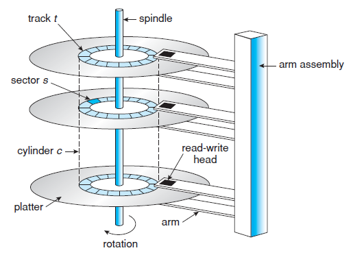
Information on a disk is magnetically recorded. The disks turn on the spindle (order of 15,000rpm). The arms do not move independently, they all move together. A disk has many concentric circles on the platter called tracks, on which a basic unit is a sector: on a disk, you cannot read or write a single byte, you can only work with a full sector at a time (which is usually around 512B).
Interface
The disk interface is thus:
readSector(logical_sector_number, buffer)writeSector(logical_sector_number, buffer)
The logical sector number is a function of the platter, cylinder or track, and sector. The main task of the file system is to translate from user interface methods to disk interface methods (e.g. from read to readSector).
Performance
To access the disk, we need to do:
- Head selection: select platter. This is very cheap (ns), and it’s just an electronic switch (multiplexer)
- Seek: move arm over cylinder. This is very expensive (few ms), as it is a mechanical motion. The cost of a seek is approximately linear in the number of cylinders that you have to move over.
- Rotational latency: move head over sector. This is also expensive (15000 RPM, half a revolution to do on average, so around 2ms)
- Transfer time: disk throughput is around 1GB/s (maybe hundreds of MB/s), so it’s cheap (microseconds)
Caching
The above is slow, so rule number one of optimizing disk access is to not access the disk: as much as possible, use main memory as a cache. To do this, keep recently acccessed blocks in memory to reduce latency and disk load by reserving kernel memory for cache; cache entries are file blocks. There are two strategies associated with this:
- Write-through: write to cache, write to disk, return to user
- Write-back: write to cache, return to user, and later, write to disk
Write-back (also called write-behind) has better much response time (microseconds vs ms), but in case of a crash, there’s a window of vulnerability that write-through doesn’t have. Still, because of the performance impact, Linux chose write-back with a periodic cache flush, and provides a primitive to flush data.
Read-ahead
Still, if you have to use disk, rule number two is don’t wait for the disk. Prefetching allows us to put more blocks in the buffer cache than were requested, so that we can avoid disk IO for the next block; this is especially useful for sequential access (which most accesses are). Note that this does not reduce the number of disk IOs, and could actually increase them (for non-sequential access). Still, in practice it’s usually a win, and in Linux, this is the default: it always reads a block ahead.
fadvise(2) allows an application to tell the kernel how it expects to use a file so that the kernel can choose an appropriate read-ahead and caching strategy. The following values can be supplied as parameters:
FADV_RANDOM: expect accesses in random order (e.g. text editor)FADV_SEQUENTIAL: expect accesses in sequential order (e.g. media player)FADV_WILLNEED: expect accesses in the near future (e.g. database index)FADV_DONTNEED: do not expect accesses in the near future (e.g. backup application)
Since Linux 2.4.10, the open(2) syscall accepts an O_DIRECT flag (a controversial addition). When Direct I/O is enabled for a file, data is transferred directly from the disk to user-space buffers, bypassing the file buffer cache; read-ahead and caching is disabled. This is useful for databases, who probably want to manage their own caches.
Disk scheduling
Now, for times that we are actually reading, we can implement rule number three which is to minimize seeks by doing clever disk scheduling. There are different disk scheduling policies:
- FCFS first-come-first-served: serve requests in the order that they were requested
- SSTF shortest-seek-time-first: pick “nearest” request in queue; note that this can lead to starvation (far-away request may never be served), but leads to very good seek times
- SCAN: continue moving head in one direction, and pick up request as we’re moving. Also called the elevator algorithm, as the head goes up and down.
- C-SCAN: similar to SCAN, but the elevator only goes one way. From cylinders
0toMAX_CYL, we pick up requests, and then going down fromMAX_CYLto0we don’t serve any. This leads to more uniform wait times. - C-LOOK: similar to C-SCAN, but instead of moving the head over the whole cylinder range, we only move it between the minimum and maximum in the queue
In practice, a variation of C-LOOK is most common.
Disk allocation
Finally, we have a final rule; rule number four is to minimize rotational latency by doing clever disk allocation. The idea here is to locate consecutive blocks of a file on consecutive sectors in a cylinder.
When we’re under low load, it works best to do disk allocation; under high load, disk scheduling works better. This is because under high load, we get many good scheduling opportunities, while allocation typically gets defeated by interleaved access patterns for different files. Under low load, we have few requests in the queue and thus few scheduling opportunities; we also tend to see more sequential access, so it makes sense to optimize for that.
OS File System Implementation
Introduction
The file system has two main functionalities: the naming/directory system, and the storage (on-disk and in-memory data structures). In this class, we’ll mainly focus on storage, because once we have this, directories can be trivially implemented by using a file to store directories.
As we’ve said before, the main task of the file system is to translate from user interface methods (read(ui, buffer, bytes)) to disk interface methods (readSector(logical_sector_number, buffer)). To study this, we’ll introduce two small simplifications. First, we’ll simplify read, which normally allows to read an arbitrary number of bytes, to only allow reading a block at a time. A block is fixed size; typically, a block is (sector size) × 2n (for instance, 4KB block size and 512B sector size). Second, for simplicity, we’ll just assume that a block is the same size as a sector.
A terminology note: the word pointer is often used, and it means a disk address (i.e. logical_sector_number), not a memory address.
Disk structure
The disk consists of a few data structures:
- Boot block: it’s at a fixed location on disk (usually sector 0); it contains the boot loader, which is read on machine boot.
- Device directory: a fixed, reserved area on disk. It’s an array of records (called “device directory entries”, DDE). It’s indexed by a
uid, and each DDE record contains information about itsuids (in-use bit, reference count, size, access rights, disk addresses). - User data: can be allocated in different ways, as we’ll see below
- Free space
Data allocation
User data can be allocated in a number of ways:
- Contiguous: disk data blocks continuous on disk. With this, we only need one pointer per device directory entry, as well as the length of the block. This creates disk fragmentation (many unusable holes) and is generally quite impractical

The DDE only contains a single pointer to the start of the contiguous data blocks - Linked list: each data block contains a pointer to the next. We only need one pointer in the DDE (2 if we store the tail), to the first data block. But this is inefficient, especially for random access, because it may require reading many blocks before getting to the right one; additionnally, it’s not great because we have a pointer taking up space in the block (and now usable block sizes aren’t a power of 2 anymore)
The DDE contains a pointer to the first data block, and every data block has a pointer to the next one - Indexed: N pointers in DDE, pointing to data blocks. The problem here is size: you can’t represent more than N blocks.
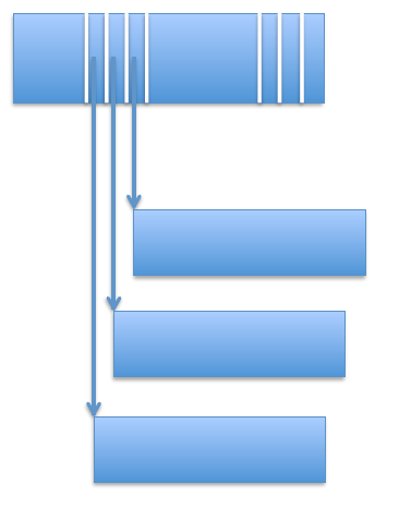
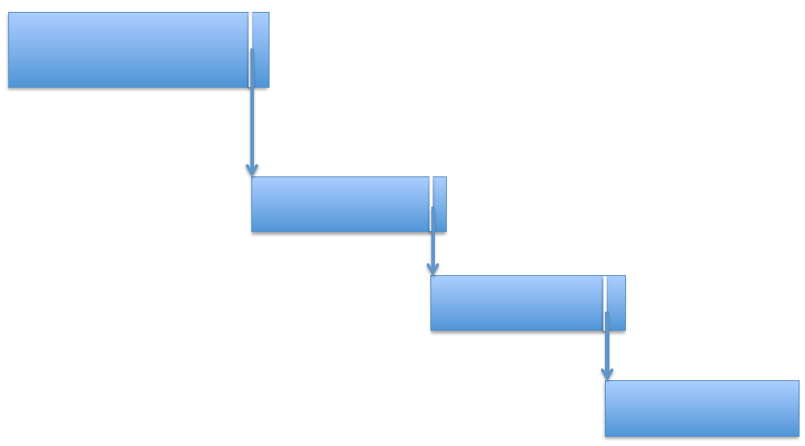
The DDE can only point to up to N data blocks - Indexed with indirect blocks: we keep the idea of N pointers in the DDE, but with a twist: the M first pointers in the DDE point to files, while the last N-M pointers point to other blocks that can point to files (or blocks). This is optimized for small files (they can be fully represented in the first block level), but also works well for large files (they can be represented in deep block levels). This can be seen as an unbalanced tree (as opposed to a full tree).
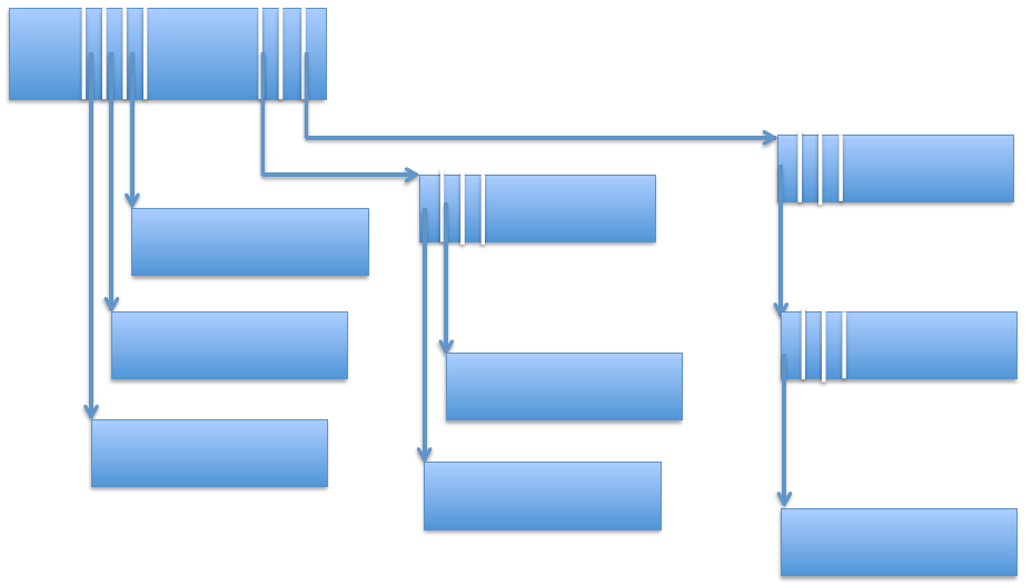
This example shows direct indexing (left), first-level indirection (middle) and second-level indirection (right) - Extent based: the DDE contains a pointer as before, but we also store the length of the extent (a small integer). In other words, in this model, the DDE points to a sequence of disk blocks. This does even better than the above, offers good sequential and random access, and can be combined with indirect blocks. This is common practice in Linux.
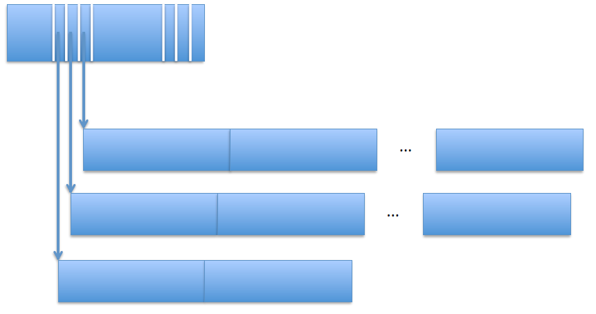
The DDE contains pointers to contiguous blocks, as well as the length of these contiguous sections
One final word: we also need to keep track of free space. This can be done with a linked list or a bitmap, which is an array[#sectors], with single-bit entries representing whether the sector is free or in-use.
In-memory data structures
-
Cache: a fixed, contiguous area of kernel memory is used as a cache. Its size is m×n, where m is the max number of cache blocks, and n is the block size. This usually makes up a large chunk of memory.
-
Cache directory: usually a hash table, where the index is given by
hash(disk address), with an overflow list for collisions. It usually has a dirty bit. -
Queue of pending user requests
-
Queue of pending disk requests
-
Active file tables: an array for the whole file system, with an entry per open file. Each entry contains the device directory entry of the file, and additional information.
-
Open file tables: an array per process, with an entry per open file of that process. It’s indexed by the file descriptor
fd. Each entry contains a pointer to the entry in the active file table, the file pointerfp, and additional information.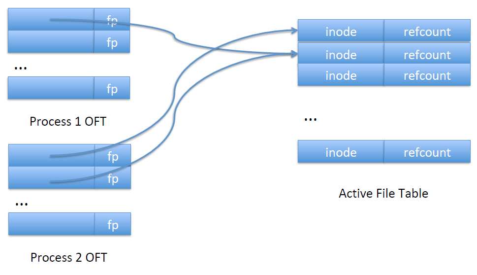
An inode is a data structure on a filesystem on Linux and other Unix-like operating systems that stores all the information about a file except its name and its actual data (source).
Pseudo-code
Putting all together, the pseudo-code of the file system primitives looks like this (with some major simplifications, since we omit permission checks, return value checks, etc):
def create():
    find a free uid (with refcount = 0) # device directory is cached; this is usually easy
    set refcount = 1
    fill in additional info
    write back to cache (and eventually to disk)
    return uid

def delete(uid):
    find inode
    refcount--
    if refcount == 0:
        free all data blocks and indirect blocks
        set entries in free space bitmap to 0
    write back to cache (and eventually to disk)

def open(uid):
    check in active file table if uid already open
    if so:
        refcount++ # in active file table
        allocate entry in open file table
        point to entry in active file table
    else:
        find free entry in active file table
        read inode and copy in active file table entry
        refcount = 1
        allocate entry in open file table
        point to entry in active file table
    fp = 0
    return tid

def read():
    find fp in open file table and increment
    compute block number to be read
    find disk address in inode in active file table
    look up in cache directory (disk address)
    if present:
        return
    else:
        find free entry in cache
        readSector(disk addr, free cache block)

def write():
    find fp in open file table and increment
    compute block number to be written
    find / allocate disk address in Active File Table
    Look up in cache directory (disk address)
    if present:
        overwrite
    else:
        find free cache entry
        overwrite

def lseek(tid, new_fp):
    in open file table, set fp = new_fp
In the pseudo-code above, we don’t write synchronously to disk; we typically use cache writeback. This is fine for user data, but for metadata, we write to disk more aggressively. Note that this does affect the integrity of the file system!
Inodes contain a reference count (or refcount for short) because of hard links. The refcount is equal to the number of DDEs referencing the inode; if we have hard-linked files, we’ll have multiple DDEs referencing a same inode. The inode cannot be removed until no DDEs referencing it are left (refcount == 0) to ensure filesystem consistency.
Loose ends
For memory cache replacement, we keep a LRU list. Unlike with memory management, this is easy to do here; file accesses are far fewer than memory accesses. Again, replacing the clean block is usually preferred, if possible. Periodically (say, every 30s, when the disk is idle), we also flush the cache.
Directories are stored as files. The only difference is that you cannot read them, only the OS can.
A very common sequence of operations is an open followed by a read; this executes a directory lookup, inode lookup and disk read for data, which means that the disk head moves between directories, inode and data for a simple read. Since this is such a common pattern, how to do this properly been a subject of research for a long time: we want these operations to be efficient, so if possible, in the same “cylinder group”, next to each other. We won’t look into this more than this in this class, but just know that it is a thing.
For file system startup, in a perfect world, no special actions are necessary. But sometimes, things aren’t normal: the disk sector can go bad, the FS can have bugs… Therefore, it’s common to check the file system. Linux has a utility called fsck (file system check) that checks that no sectors are allocated twice, and that no sectors are alloacted and on free list (this could happen in the case of a crash happening between freeing). Effectively, fscheck reconstructs the free list instead of trusting what is already there.
Another thing that can go wrong is that some sectors can go bad. To solve this, we do replication of important blocks, like the boot block, and in modern systems, the device directory.
Disk fragmentation happens even if we have good allocation. Over time, we’ll end up with small “holes” of one or two sectors, and files spread all over the disk. On a fragmented disk, it’s no longer possible to do good allocation. The solution is to take the FS offline, move files into contiguous locations, and put it back online (you can do it without taking the FS down, but it’s tricky and not advisable).
Alternative file access method: memory mapping
There are alternative file access methods: mmap() maps the contents of a file in memory, and munmap() removes the mapping. This is the real reason why people wanted 64 bit address spaces: if you mmap a few big files, you’re out of address space really fast! (The reason wasn’t that the heap ran into the stack, or that the code got too big for 32 bits, it’s mainly a mmap problem). With 64 bits, there is ample space between the heap and the stack for mmap-ed files.
To access mmap-ed files, we access the relevant memory region, page fault, and cause the page file to be brought in.
mmap():
    allocate page table entries
    set valid bit to "invalid"
    on read:
        page fault
        # just like in demand paging:
        file = backing store for mapped region of memory
        set valid bit to "valid"
    on write:
        write to memory
Page replacement will take care of getting the data to disk (we can also force it through msync()). mmap is very good for small, random accesses to big files (in databases, for instance), as it only brings the data we need into memory. It’s also an easier programming model than lseek and read, and it’s easier to reuse data this way.
But there are restrictions too: you can only mmap on a page boundary, it’s not easy to extend a file, and for small files, reads are usually cheaper than the mmap + page fault. Indeed, for random access to small files, it may be better to read the whole file into memory first.
Another use of mmap is for sharing memory between processes, as a form of interprocess communication (through shared, anonymous map flags).
Dealing with crashes
Atomic writes
Crashes can happen in the middle of a sequence of writes, and it can have catastrophic effects. Therefore, we aim for atomicity: it’s all or nothing. In a file system, that means that either all updates are on disk, or no updates are on disk; we do not allow for in-betweens. How can we make sure that all or no updates to an open file get to disk?
We’ll operate under the assumption that a single sector disk write is atomic (which is 99.99999…% true. Disk vendors work very hard at this, we’ll just assume it’s always true).
To switch atomically from old to new, we cannot write in-place. Instead, we write to new, separate blocks on the disk, and switch the pointer in the DDE atomically. Old blocks are then de-allocated. If the crash happens before they’re de-allocated, the file system check will fix it.
A more precise description of this process follows: when opening, we read the DDE into the AFT, which effectively creates a copy of the (on-disk) DDE in memory. For writes, we allocate new blocks for the data, write these addresses into the incore DDE, and write to cache. On close, we write all cached blocks to disk blocks, and atomically write the DDE to disk.
Intentions log
An alternative method is the intentions log. We reserve an area of disk for the intentions log.
def write():
    write to cache
    write to log
    make in-memory inode point to update in log

def close():
    write old and new inode to log in one disk write
    copy updates from log to original disk locations
    when all updates are done, overwrite inode with new value
    remove updates, and old and new inodes from log
On recovery from a crash (in other words, on any reboot, since we can’t know if we’ve crashed or not), we search through the log, and for every new inode found, we find and copy the updates to their original location. If all updates are done, we write to the new inode, and then remove updates and old and new inodes from log.
If the new inode is in the log and we crash, then we’ll end up with the new inode. If it isn’t, then we keep the old one. This works even if we crash during crash recovery.
Comparison
The DDE method has one disk write for write(), and one for close(). Log does two disk writes for write() (one to the log, another for the data), and one for close(). And yet surprisingly, log works better! That’s because writes to the log are sequential, so we have no seeks. Data blocks stay in place, and disk allocation stays. To further optimize this, we can write from cache or log to data when the disk is idle, or during cache replacement.
With DDE, disk allocation gets messed up, and we have high fragmentation.
All modern OS file systems implement log-based systems.
Log-Structured File System (LFS)
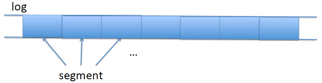
This is an alternative way of structuring the file system, which takes the idea of the log to the extreme. The rationale is that today, we have large memories and large buffer caches. Most reads are served from cache anyway, so most disk traffic is write traffic. So to optimize I/O, we need to optimize disk writes by making sure we write sequentially to disk. The key idea in LFS is to use the log, an append-only data structure on disk.
Writing
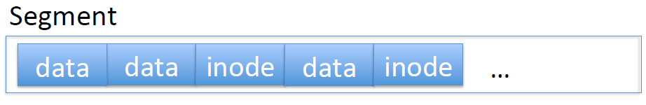
All writes are to a log, including data and inode modifications. Writes first go in a cache, and are eventually written with writeback. Writes also go into an in-memory buffer. When it’s full, we append it to the log: that way, we add to the log in blocks called segments. Since we’re adding sequentially, we don’t do any seeks on write.
A single segment contains both data and inode blocks, and the log is a series of segments.
Reading
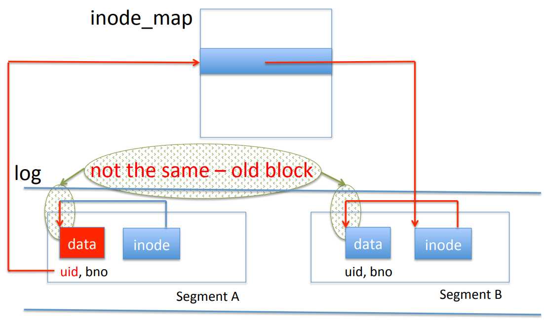
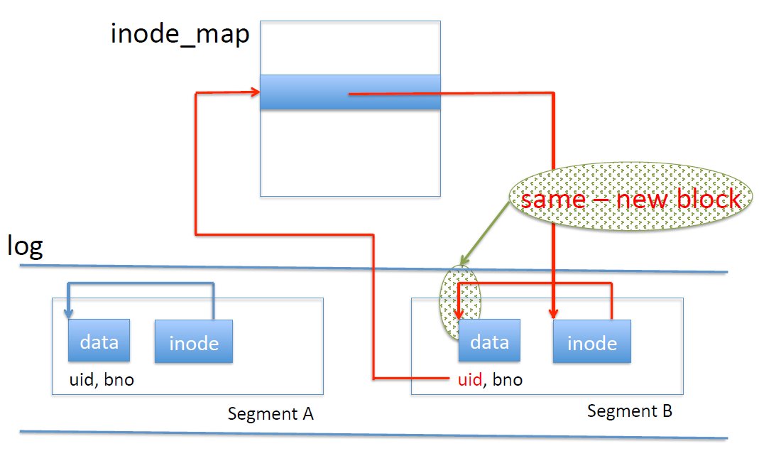
When we write an inode, we write it to the inode map; this is an in-memory table of inode disk addresses:
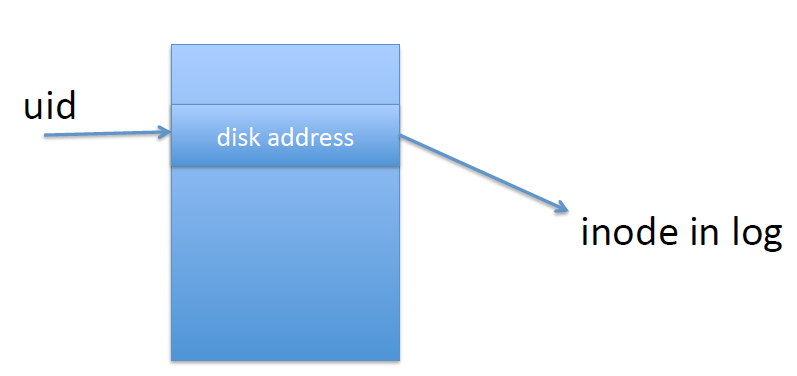
The inode map holds the following mapping: uid -> disk address of the last inode for that uid
To read, we need to go through the indirection of the inode map:
def open():
    get inode address from inode map
    read inode from disk into active file table

def read(): # as before
    get from cache
    get from disk address in inode
With the added indirection of the inode map, reading seems more complicated; but performance is chiefly determined by disk reads, so at the end of the day, there is little difference.
Checkpoints
How do we get the inode map to disk? We do what’s called a checkpoint: we write a copy of the inode map to a fixed location on disk, and we put a marker in the log.
Fake news alert: we said “all data is written to the log”, but in reality, it’s “all except for checkpoints”.
On a crash, we start from the inode map in the checkpoint. This contains addresses of all inodes written before the last checkpoint. To recover, we need to find the inodes that were in the in-memory inode map before the crash, but not yet written in the checkpoint. To do this, we “roll forward”. Remember that the checkpoint put a marker in the log: from this marker forward, we scan for inodes in the log, and add their addresses in to the inode map.
We need to pick a time interval between checkpoints. Too short, and we’ll have too much disk I/O; too long, and the recovery time will be too long (the forward scan can be slow). The compromise is based on the assumption that crashes are rare (if they aren’t, you should probably buy another machine), so we can err towards larger time intervals. The compromise is typically on the side of long recovery times (there are exceptions for critical applications; if your OS is controlling a plane, then you probably want recovery time to be fast, so that the plane doesn’t crash because of forward scanning).
Disk cleaning
What if the disk is full? We always write to the end of the log, never overwriting. This means that the disk gets full quickly. Therefore, we need to clean the disk. In this process, we reclaim old data. In this context, “old” means logically overwritten but not physically overwritten. Data is logically overwritten when there’s a later write to the same (uid, blockno) in the log; it is physically overwritten once it’s been committed to disk (so if there’s an older version of (uid, blockno) in the log, it’s not physically overwritten yet).
Disk cleaning is done one segment at a time. We determine which blocks in the segment are new, and write them into a buffer; when the buffer is full, we add it to the log as a segment. The cleaned segment is then marked free.
How do we determine whether a block is old or new? We actually have to modify write() a little. Instead of only writing data to the buffer and log, we must write data, uid and blockno. With this, for a given block, we can take its disk address, its uid and blockno, and look them up in the inode map. This gives us an inode; if it has a different address, then it must be old. Otherwise, it must be new.
Taking cleaning into account, the log actually is more complicated than a simple linear log. It’s actually a sequence of segments, some in use, some free. Writes thus don’t only append to the log, but typically write to a free segment.
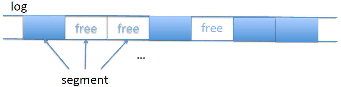
But the whole point of the log is sequential access so that we never have to move the head! This is true, but the segments tend to be very large (100s of sectors, MBs), so we tend to still get large sequential accesses with the occasional seek. This stays rare, so performance is still very good.
Summary
In summary, LFS reads mostly from cache. The writes to disk are heavily optimized, so we have very few seeks. The reads from disk are a bit more expensive, but it’s not so bad, since there are few of them. With LFS, we have to endure the cost of cleaning.
The checkpoint and the log are on disk; the checkpoint region is at a fixed location, and the log uses the remainder of the disk. Individual segments in the log contain data and inode sectors, where data includes uid and blockno.
Additional in-memory data structures assist us in this system: the cache is a regular write-behind buffer cache, and the segment buffer is for the segment currently being written, which goes to the log all at once when it’s full. The inode map is a map indexed by uid pointing to the last-written inode for uid. In addition to this, we also have the active and open file tables, as before.
Writes put data and inodes into (write-back) cache and in-memory segment buffer, which goes to a free segment in the log once it’s full, which means almost no seeks on write! To open, we read the inode map map to find the inode, and read the inode into the active file table. To read, we get from cache; if it isn’t there, we must get from disk using the disk address in the inode, as before.
LFS is actually more complicated than we presented, but has not become mainstream. This is mainly because cleaning has a considerable cost, and causes performance dips (and people like systems that are predictable). On top of that, the complexity of this system makes it very difficult to implement the code for it. Still, there are similar ideas in some commercial systems (especially high-throughput systems, like computing clusters).
What has become popular are journaling file systems, that use a log (called a journal) for reliability (we can cite ext4 in Linux).
Note that cleaning is somewhat similar to garbage collection, both in its function and its effects. But cleaning happens on disk (as opposed to in memory), and is much slower.
Alternative storage media
Since the 1970s disks have improved by a factor 100 to 1000 in terms of physical size, cost and capacity. But bandwidth and latency of disks, the two most important factors for performance, have lagged behind, only improving 10-fold. This is problematic for servers, big data computations, transaction systems, etc.
There are two developments that have risen as a response to this: RAID and SSDs. They both improve performance, but remain more costly than disks.
RAID
RAID stands for “Redundant Array of Independent Disks”. The main concept behind RAID is striping: rather than put a file on one disk, we stripe it across a number of disk. The idea here is that if you put all your data on one disk, the bandwidth isn’t so good, but you can parallelize this: in the best of worlds, the bandwidth of n disks is n times the bandwidth of a single disk. There are other factors that put a cap on this (bandwidth of IO bus, controller, etc), but essentially this holds.
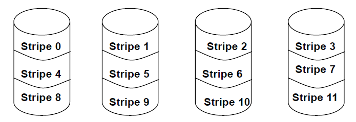
The downside here is that one disk fail makes all data unavailable. When talking about disk failures, the main figure is MTBF (mean time between failures), which is typically 50,000 hours (5 years). But for RAID disks, it’s the MTBF of a single disk, divided by n. So for 10 disks, we’re looking at half a year, which is clearly not acceptable.
That’s why RAID also has a notion of redundancy. RAID comes with a RAID level of redundancy. What we described above is RAID-0, i.e. no redundancy. But in reality, people use RAID-1 (mirroring), RAID-4 (parity disk), or RAID-5 (distributed parity).
-
RAID-0: offers the best possible read and write bandwidth, the lack of redundancy makes failures result in data loss, which is typically not acceptable.
-
RAID-1: we keep a full mirror (back-up) of all the data. Writes must go to both data and mirror disk, but reads may go to any of them. After a crash, we recover from the surviving disk. But in this process, we’ve also halved storage capacity for the same number of disks as RAID-0; we can do better.
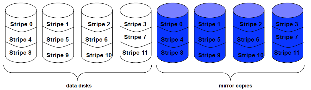
- RAID-2: practically never used in practice; stripes data at the bit level (instead of block level), and uses a Hamming code stored across at least 2 additional drives for error correction. The added complexity of Hamming codes offers no significant advantage over the simpler parity bits (it can repair undetected transient errors on a single bad bit, which other levels cannot do, but at the cost of an extra drive), so RAID 2 has rarely been implemented.
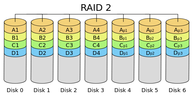
Source: Wikipedia, CC-BY-SA 3.0 -
RAID-3: practically never used in practice; stripes data at the byte level (instead of block level), is able to correct single-bit errors, and uses a dedicated parity disk. Because it stripes at the data level, any single block I/O is spread on all disks, meaning that RAID-3 cannot service multiple requests simultaneously.
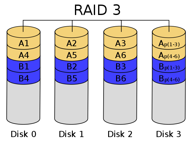
Two six-byte blocks (in different colors) and their two parity bytes. Source: Wikipedia, CC-BY-SA 3.0 -
RAID-4: N data disks and 1 parity disk. Parity is a simple form of error detection and repair (not specific to RAID, also used in communications). A parity bit is computed as the XOR of 4 bits: p = a ⊕ b ⊕ c ⊕ d. If we lose a bit, say bit b, we can reconstruct it as b = a ⊕ c ⊕ d ⊕ p. In RAID-4, we use the same idea at the disk block level; the parity disk holds the XOR of the bits of data blocks at the same position. Reads read from data disks, while writes must write to data and parity disks. On a crash, we can recover using the parity disk and the other disks.
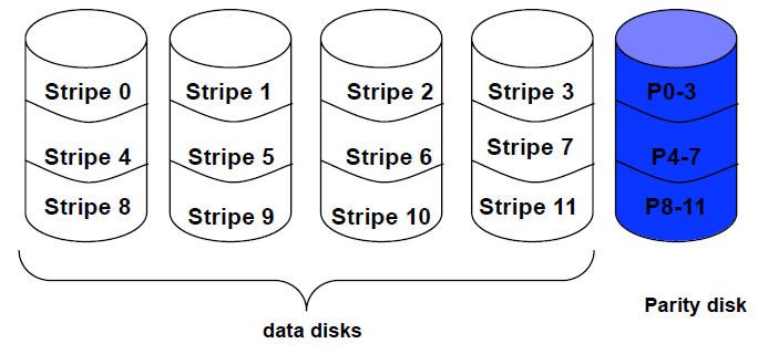
The issue is that every write implies an additional access to a parity disk, which quickly becomes a bottleneck for write-heavy workloads; we can do better.
-
RAID-5: just like RAID-4, but we distribute the parity blocks over all disks; this balances parity write load over all disks.
-
RAID-6: double parity, in case of double disk failures
- RAID-1+0: RAID-0 of RAID-1 configurations
SSD
The first thing to note is that SSD (Solid State Disks) are not in fact disks. They’re a purely electronic drive (based on NAND flash), with no moving parts. The basic unit in NAND flash are pages (4K) and blocks (e.g. 64 pages).
SSDs were made to be a plug-and-play replacement for HDDs; they have the same form factor and interface as HDDs (even though they have no other technical reason to be so). The SSD interface is thus very much like a disk, with readSector and writeSector. The bandwidth is higher than disk, and the latency is much lower (order of 100 μs for read, 300 μs for write).
Basic operations are:
read(page)write(page): note that we cannot rewrite a page, only write to a blank one (see below)erase(block): we must erase a block before a page can be rewritten to. There’s a limited number of erase cycles that SSD manufacturers guarantees (order of 100,000)
Since a block must be completely erased before any single page in a block is written, we write pages sequentially in a block. We cannot overwrite, but need to erase a block before writing. This should remind of us LFS… and indeed, an LFS-like system is perfectly suited for SSDs.
With LFS, we can clean the block before erasing, move live data to a new block, and erase it. To do this, we have the TRIM command, TRIM(range of logical sector numbers) to indicate to the device that some sectors are no longer in use. If that’s been called, then there’s no need to do cleaning, we can just trust what we’ve been told and erase without checking.
Still, when we do cleaning, our strategy when picking blocks is to even out the number of erase cycles, in an attempt to extend the longevity of the SSD.
Virtual Machines
Virtualization
Virtualization is an instance of indirection, and to be more specific, of layering.
“Any problem in computer science can be solved with another layer of indirection. But that usually will create another problem.”
— David Wheeler
There are three mechanisms of virtualization:
- Multiplexing: take one resource, and expose it as multiple virtual entities. Each entity appears to have the full resource (e.g. virtual memory on the MMU)
- Aggregation: take multiple resources, and expose it as a single virtual entity. The goal is typically to achieve enhanced properties, be it bandwidth, capacity, availability, redundancy… A canonical example for this is RAID.
- Emulation: make a resource appear as a different type of resource. For instance, use software to emulate a virtual resource which is different from the underlying physical resource. Examples include RAM disks, Android Emulator or the JVM (which is simply emulating a different instruction set)
Terminology
A virtual machine (VM) is virtualiization applied to an entire computer: a machine running on a machine. Usually, we use virtualization to run many machines on a single machine. The real, base machine is the physical machine, and the ones running on top are virtual machines.
The VMM (Virtual Machine Monitor) is a resource manager for VM. It is comparable to the OS in the sense that they both provide resource management (between processes for an OS, between VMs for a VMM), but an OS provides abstractions (processes, address spaces, FS, …) and a VMM doesn’t; a VMM provides an identical copy of the machine.
The VMM provides creation, destruction and scheduling of VMs, and takes care of memory, disk and I/O management for VMs. Note that this is similar to what an OS does (but with processes replaced by VMs), but again, it’s not the same because a VMM doesn’t provide abstraction.
In a VM, you typically run an OS (called a guest OS), with applications on top. This is opposed to the host OS, which is the one running on the metal (as opposed to in the VM).
The hypervisor or Type I VMM is a VMM that is also a host OS (e.g. Xen, VMware vSphere, Microsoft Hyper-V), while a hosted VMM or Type II VMM is separate from the host OS (e.g. KVM, VMware Workstation and Fusion, or Parallels).
An application or OS running on real hardware runs in native mode. If it runs on virtual hardware, we say it’s running in virtualized mode.
History
As a bit of history, the VM was developed in the 1970’s by IBM. Back then, the mainframes were very expensive, and VMs allowed sharing by users running different OSes. It fell out of favor in the 80’s and 90’s as cheap microprocessors were introduced, but became prominent again in the 90’s, mainly for server consolidation (most servers are mostly idle, so to save power, we can run multiple servers on the same machine).
VMM Implementation
There are three requirements for a VMM:
- Equivalence: the virtual hardware needs to be sufficiently equivalent to the underlying hardware that you can run the same software in the virtual machine
- Safety: the VM must be completely isolated from other VMs and from the VMM. This also means that VMs cannot interfere with each other, or hog resources.
- Performance: the overhead of virtualization must be low enough that the VM can still reasonably run, i.e. that it can be used just as if it were running directly on the hardware.
How do we implement a VMM? A major problem to solve is around kernel vs. user mode, privileged instructions and system calls. In native mode, the kernel-user boundary is between applications in the OS, but where should we place it in virtualized mode?
Keeping it between the applications and the OS is incorrect; we would ruin the safety requirement because, as we saw in the beginning of this course, kernel mode is God mode. We can place the boundary between the VMM and the guest OSes, but that raises another problem: the guest OSes are now in user mode, even though they were written for kernel mode. As a result, we run into a host of problems:
- System calls (that usually put the machine in kernel mode) won’t work correctly
- Since the OS and the applications are in user mode together, the applications could access the guest OS memory
- The guest OS uses privileged instructions
We can solve the above with the following solutions:
-
If an application does a syscall, it wants to perform it in its guest OS. But the syscalls go to the VMM, which holds syscall vectors for the physical machine. But we want to access the syscall vectors for the OS in the guest OS, so the VMM must somehow forward the syscall.
Remember that hardware directs syscalls to physical syscall vectors; it puts the machine into kernel mode and jumps to the machine’s syscall handler.
Therefore, at boot time, the VMM installs physical machine syscall vectors. At guest OS boot time, the OS wants to install its syscall vectors through a privileged instruction. But being in user mode, it traps to the VMM, which will thus gain the information of where the OS syscall handlers are.
When the VMM’s syscall handler is called, it can set the PC to the appropriate syscall vector in the OS, and returns to user mode, in which the guest OS will run its syscall handler. Inevitably, this guest OS syscall handler will execute the “return to user mode” instruction, which traps to the VMM, that can set the PC to the instruction following the original syscall and return to user mode in the guest OS.
-
On switching back from the VMM to the VM, if the return address is in the guest OS, we allow all memory accesses within the VM. If it is outside the guest OS (i.e. to an application), we disallow access to the guest OS memory. This is all done through protections in the page table.
-
The solution to this is outline in the first one, but the gist of it is that privileged instructions will trap to the VMM, which will handle it (i.e. emulate the outcome of the privileged instructions) and return to the OS kernel (except for return to user mode, where we return the application). This is known as trap-and-emulate. Another solution is dynamic binary translation, where we translate a privileged instruction to an unprivileged one. But this has very high overhead and is best avoided.
Note that unprivileged instructions (from an application, but also from the OS) can be run directly, without having to pass through the VMM; they are directly sent to the metal for performance. This is called limited direct execution: we let some instructions (but not all!) run directly on the metal.
Popek/Goldberg Theorem
An instruction is privileged if it can only be executed in kernel mode. It is sensitive if it behaves differently in kernel and user mode. The Popek/Goldberg theorem states:
Note that trap-and-emulate doesn’t work if some privileged instructions don’t trap. Indeed, any privileged instruction that doesn’t trap is sensitive, and these exist in common architectures: x86 has 17 sensitive, unprivileged instructions. Writing a VMM is still possible, but it is more complicated.
In this case, we must resort to some workarounds. We could do a binary rewrite of the guest OS to remove sensitive unprivileged instructions, but this is very tricky and has high overhead. More recently though, we have solutions like Intel VT-x and AMD-v (2005, available on all 64-bit processors) which duplicate protection rings to meet the Popek/Goldberg criteria.
Virtual memory
To implement virtual memory, we use paging with valid bits.
Remember that in native mode, processes (and the processor) issue virtual addresses. The memory management unit (MMU) produces a physical address from the TLB or page table, which goes to memory. The OS allocates physical memory to processes, and installs page table and TLB entries to do so.
In virtualized mode, the VMM allocates memory between VMs, and the OS installs page tables and TLB entries to do so. The guest OS thinks it’s running on the real machine and has control over all memory of the real machine, but it is in fact running on the virtual machine and only has a limited portion (as allocated by the VMM).
To implement this, we need two levels of memory translation. The virtual address is still the virtual address (VA). What we called physical address (PA) in native mode becomes the guest physical address (gPA) in virtualized mode, and we introduce an additional address, the host physical address (hPA).
In native mode, we simply translated VA → PA. In virtualized mode, we translate VA → gPA in the guest OS (using guest TLB and guest page tables), and gPA → hPA in the VMM (using the real TLB and physical page tables). This means that we must have one guest page table per process in the guest OS, which we let reside in the guest OS memory. We also have a physical page table per VM, which resides in VMM memory.
The VA → gPA translation is done by the guest OS (remember that it doesn’t change); to allocate a new page to a process, it finds a free frame, and inserts the page-frame mapping in both page table and TLB. These insertions are privileged instructions that trap to the VMM, which will trap-and-emulate. The gPA → hPA translation is done as in the native OS before. To allocate a page to a VM, we find a free frame and insert the page-to-frame mapping in the VM’s page table, and copy the mapping over in the TLB.
This is an expensive process: we need to walk two levels of page tables. But modern processors have nested page tables available, which allows us to access the nested levels in parallel and in hardware, which reduces the cost of VM memory management.
Without nested page tables, we have a challenge: we only have one physical TLB for the whole physical machine and all of the VMs! One solution is to implement shadow page tables: we keep two copies of the guests’ page tables. The real copy is in the hardware (backed by the real TLB) and contains VA → hPA, while the shadow copy is in software and contains VA → gPA. The guest updates the shadow copy, and the VMM updates the real copy from the shadow copy.
« Back